The Fourier transform: asking a signal how much of each frequency it contains

The question

Here are thirty days of sea level at a harbor, one reading per hour.

Show code

Copy

import numpy as np
import matplotlib.pyplot as plt

plt.rcParams.update({
    "figure.dpi": 110, "axes.spines.top": False, "axes.spines.right": False,
    "axes.grid": True, "grid.alpha": 0.25, "font.size": 11, "lines.linewidth": 1.6,
})
INK, ACCENT, SECOND, MUTED = "#1f2a44", "#c8553d", "#2a7f9e", "#8a8f98"

# The record is synthetic, built from four tidal constituents plus noise, so that
# the answer can be checked at the end. Pretend you have not seen this cell.
rng = np.random.default_rng(42)
t = np.arange(0, 30 * 24, 1.0)                     # hours
constituents = {                                   # period / h, amplitude / m, phase
    "M2": (12.4206, 1.00, 0.0),
    "S2": (12.0000, 0.45, 0.7),
    "K1": (23.9345, 0.30, np.pi / 2),
    "O1": (25.8193, 0.20, 1.2),
}
h = sum(A * np.cos(2 * np.pi * t / P + phi) for P, A, phi in constituents.values())
h += 0.15 * rng.standard_normal(t.size)            # wind, waves, the instrument

fig, ax = plt.subplots(figsize=(8, 3))
ax.plot(t / 24, h, color=INK, lw=1)
ax.set(xlabel="time / days", ylabel="sea level / m", xlim=(0, 30))
plt.show()

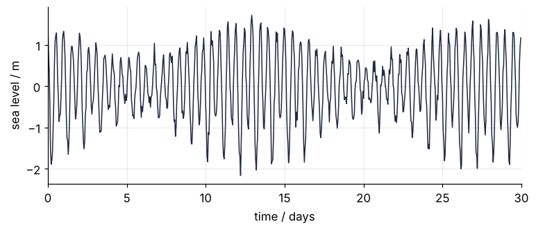
Two things are obvious. The water goes up and down about twice a day, and the swings are large for a week, then small for a week, then large again. Sailors have known both for millennia: the tide, and the fortnightly alternation of spring and neap tides.

Less obvious: how many distinct rhythms are in this record, what are their periods to three decimals, and how strong is each? The twice-daily beat is in fact two rhythms with periods 12.42 h and 12.00 h, one from the Moon and one from the Sun, and the week-long swelling is what you see when two nearly equal frequencies interfere. The Fourier transform is the instrument that takes such a record apart. This tutorial is about what it actually does, not about which function to call. That comes at the end, in six lines.

The idea: compare the signal with a probe

Suppose you want to know whether the record contains an oscillation with a period of 12 hours. Build one, a probe: \(\cos(2\pi f t)\) with \(f = 1/12\) cycles per hour. Multiply it with the signal, point by point, and take the average of the product.

If the signal contains that rhythm, signal and probe rise together and fall together. Their product is positive most of the time, and the average comes out clearly different from zero. If the signal does not contain it, the product is positive about as often as it is negative, and the average is close to zero. Here are three probes, slightly below, at, and slightly above the lunar period of 12.42 h, on the first three days of the record:

Copy

def probe_average(f):
    """Average of signal times a cosine probe, scaled so that it reads as an amplitude in m."""
    return 2 * np.mean(h * np.cos(2 * np.pi * f * t))

window = t < 72
fig, axes = plt.subplots(3, 1, figsize=(8, 6.5), sharex=True)
for ax, f in zip(axes, [0.0700, 1 / 12.4206, 0.0900]):
    probe = np.cos(2 * np.pi * f * t)
    ax.plot(t[window], h[window], color=INK, label="signal")
    ax.plot(t[window], probe[window], color=SECOND, lw=1, label="probe")
    ax.fill_between(t[window], 0, (h * probe)[window], color=ACCENT, alpha=0.35, lw=0, label="product")
    ax.set_ylabel("m")
    ax.text(0.99, 0.92, f"f = {f:.4f} /h   average = {probe_average(f):+.2f} m",
            transform=ax.transAxes, ha="right", va="top")
axes[0].legend(frameon=False, loc="upper left", ncol=3)
axes[-1].set_xlabel("time / h")
plt.show()

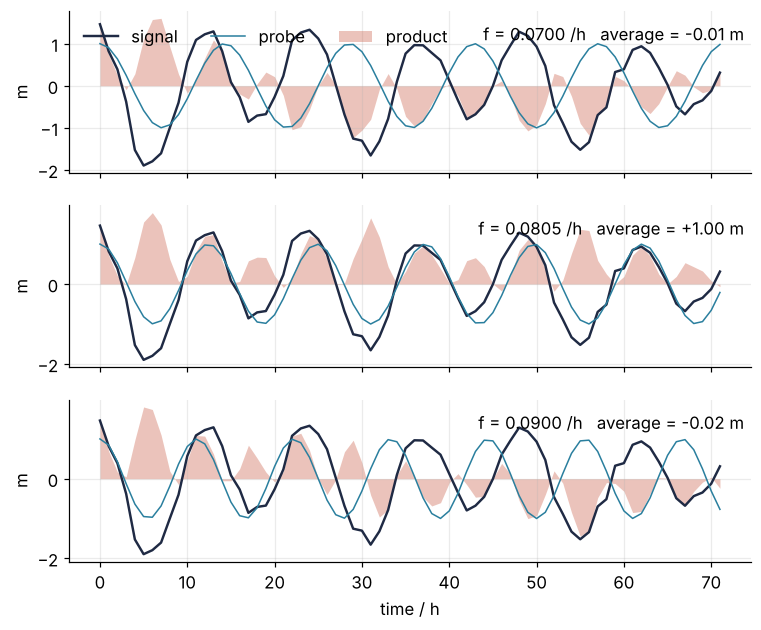
At 0.0700 cycles per hour the shaded product changes sign every few hours and averages to almost nothing. At the lunar frequency, the product is mostly positive and averages to 1.00 m. At 0.0900 it is gone again. The probe has found the rhythm and its amplitude.

Now sweep the probe frequency continuously and plot the average against it. That is the whole idea. Watch the spectrum being traced out:

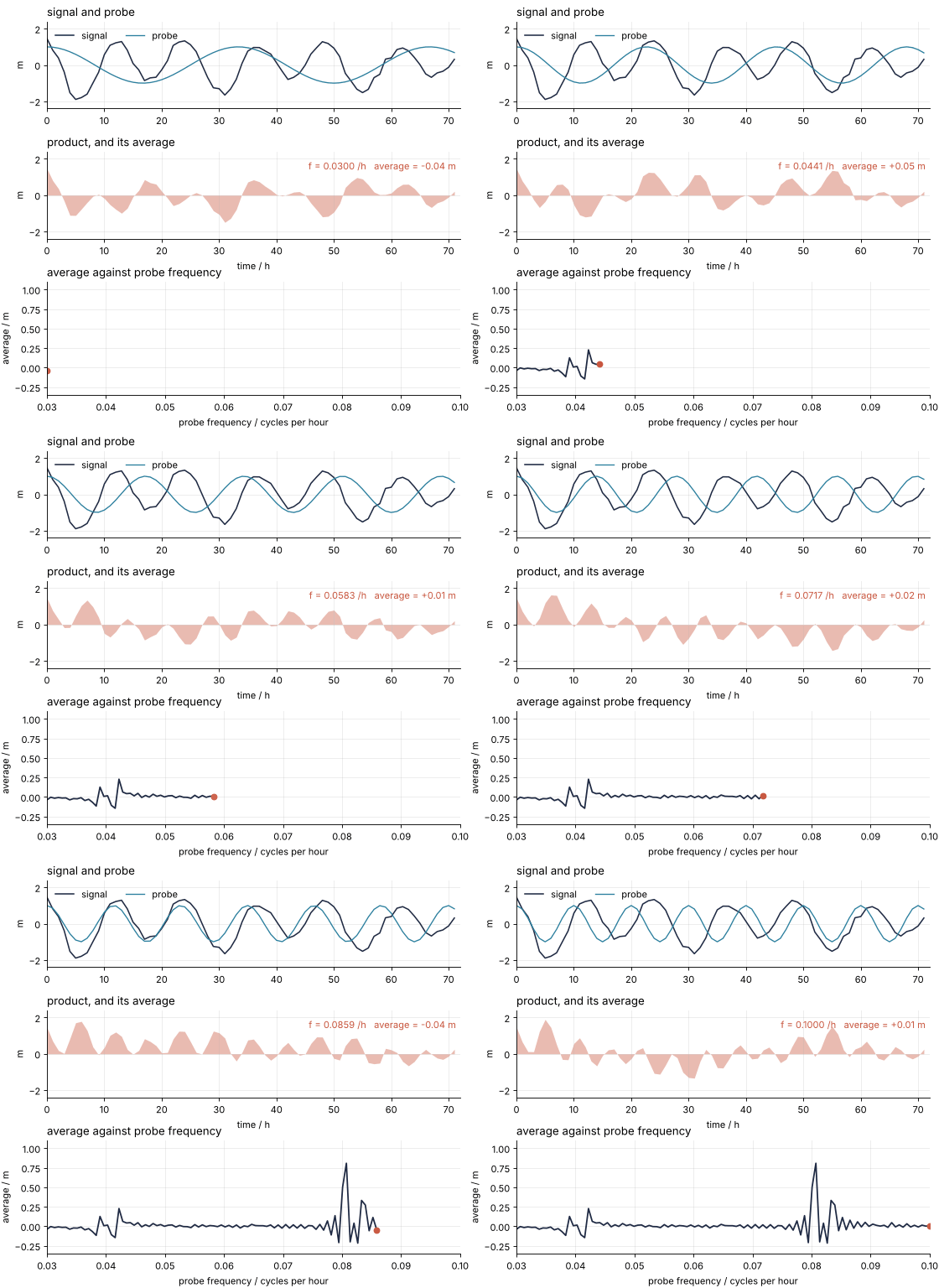
How I built this: Visualization tutorial "Animating a probe sweep", planned.

Copy

f = np.linspace(0.01, 0.12, 2000)
cos_sweep = np.array([probe_average(x) for x in f])

fig, ax = plt.subplots(figsize=(8, 3.2))
ax.plot(f, cos_sweep, color=INK)
ax.set(xlabel="probe frequency / cycles per hour", ylabel="average / m")
plt.show()

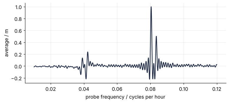
Two peaks at 0.0805 and 0.0833 cycles per hour, that is at 12.42 h and 12.00 h, and a wobble around 0.04. But the plot has a problem. We know from the first figure that the water level also has a daily component. Where is it?

The lost phase, and why the transform is complex

The probe is a cosine. A rhythm in the signal that happens to be a sine, a quarter period out of step with the probe, gives a product that is positive for a quarter period and negative for the next, and averages to exactly zero. The daily rhythm in this record is such a case. The cosine probe sees it only as that antisymmetric wobble around 0.04, which crosses zero exactly where the peak should be. The second daily component is seen at a fraction of its true strength, depending on its phase.

The fix is to probe with a cosine and a sine at the same time and keep both results. Euler's formula packs the pair into one complex number, \(e^{-2\pi i f t} = \cos(2\pi f t) - i\sin(2\pi f t)\), so the two averages become the real and imaginary part of a single complex average. Its magnitude is the amplitude of the rhythm, whatever its phase, and its angle is the phase. That is all the complex numbers in the Fourier transform are: a way to carry two probes in one symbol.

Copy

def spectrum(f):
    """Magnitude of the complex probe average: the amplitude at frequency f, in m."""
    return 2 * np.abs(np.mean(h * np.exp(-2j * np.pi * f * t)))

amp = np.array([spectrum(x) for x in f])

fig, ax = plt.subplots(figsize=(8, 3.2))
ax.plot(f, amp, color=INK)
for name, (P, A, phi) in constituents.items():
    ax.annotate(name, (1 / P, A), xytext=(0, 6), textcoords="offset points", ha="center", color=ACCENT)
ax.set(xlabel="probe frequency / cycles per hour", ylabel="amplitude / m", ylim=(0, 1.15))
plt.show()

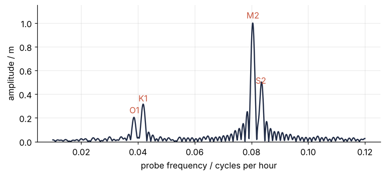
Four peaks now, two around a day and two around half a day, with heights of 1.00, 0.50, 0.32 and 0.20 m. The labels are the names oceanographers give these constituents. M2 is the Moon's principal tide, S2 the Sun's, K1 and O1 are the two daily ones. The record was made of exactly these four, with amplitudes 1.00, 0.45, 0.30 and 0.20 m, and the amplitude spectrum has read them back off, including the one the cosine probe could not see. S2 reads 0.50 instead of 0.45 because the skirt of the much stronger M2 peak next to it adds to its height; the next section says why peaks have skirts at all.

Formalization

What we have been computing is, up to the normalization, the Fourier transform. For a signal \(x(t)\),

\(|X(f)|\) is the strength of frequency \(f\) in the signal and \(\arg X(f)\) its phase. The transform is invertible: \(x(t) = \int X(f)\, e^{+2\pi i f t}\, df\) rebuilds the signal from its frequencies, which says that any reasonable signal is a sum of oscillations and \(X\) tells you the recipe.

For a record of \(N\) samples \(x_n\) taken at spacing \(\Delta t\), the integral becomes a sum,

the discrete Fourier transform. A cosine of amplitude \(A\) in the signal produces \(|X_k| = N A / 2\) at its frequency, which is why the code above multiplies by \(2/N\) to read amplitudes in meters. The reason it works is a trigonometric identity: the product of two cosines is half the cosine of the difference frequency plus half the cosine of the sum frequency. The sum term oscillates and averages away. The difference term also averages away, unless the frequencies agree, in which case it is a constant, \(A/2\). The factor of two undoes the half.

The discrete version has two consequences you need every time you use it.

Resolution. The frequencies \(f_k\) are spaced by \(1/(N\Delta t) = 1/T\), the inverse of the record length. Two rhythms closer than \(1/T\) land on the same point of the spectrum and cannot be told apart. M2 and S2 differ by \(1/12.00 - 1/12.42 = 0.00282\) cycles per hour, so separating them needs a record longer than \(1/0.00282 = 355\) hours, or 14.8 days. That number should sound familiar: it is the spring–neap period, the beat between the two. You cannot resolve two frequencies until you have watched them go through one full beat against each other. Here is the same spectrum computed from the first seven days only:

Copy

def spectrum_of(x, tx, f):
    return np.array([2 * np.abs(np.mean(x * np.exp(-2j * np.pi * fi * tx))) for fi in f])

f_zoom = np.linspace(0.07, 0.095, 800)
week = t < 7 * 24

fig, ax = plt.subplots(figsize=(8, 3.2))
ax.plot(f_zoom, spectrum_of(h, t, f_zoom), color=INK, label="30 days")
ax.plot(f_zoom, spectrum_of(h[week], t[week], f_zoom), color=ACCENT, label="7 days")
for name in ["M2", "S2"]:
    ax.axvline(1 / constituents[name][0], color=MUTED, lw=1, ls="--")
ax.set(xlabel="frequency / cycles per hour", ylabel="amplitude / m")
ax.legend(frameon=False)
plt.show()

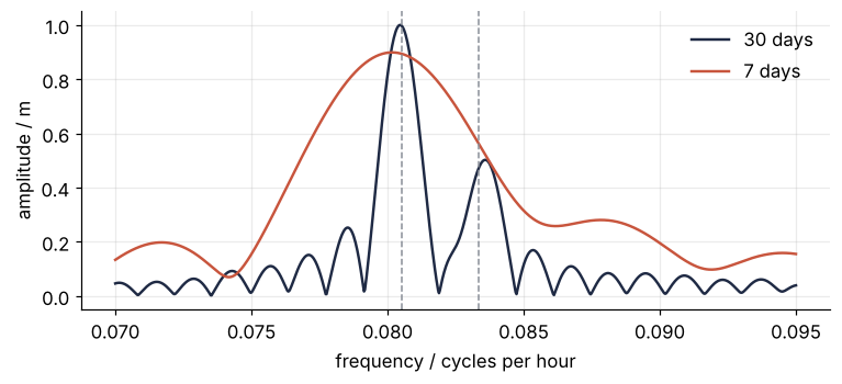
With one week of data the two semidiurnal tides merge into a single broad bump. No amount of cleverness recovers them from that record; the information is not in it.

The highest frequency you can see. With samples every \(\Delta t\), the spectrum is only meaningful up to \(f = 1/(2\Delta t)\), the Nyquist frequency. Anything faster is folded back onto a lower frequency and shows up as a false rhythm. Hourly readings resolve periods down to two hours, which is plenty for tides. A 1 Hz sensor cannot tell you anything about a 3 Hz vibration, except by lying.

See it in code

The sweep above evaluates the sum for every probe frequency separately, which is slow for large records. The fast Fourier transform computes all \(X_k\) at once in \(N \log N\) operations, and NumPy provides it. For a real-valued signal use rfft, which skips the redundant negative frequencies:

from scipy.signal import find_peaks

X = np.fft.rfft(h)
freq = np.fft.rfftfreq(t.size, d=1.0)          # cycles per hour; d is the sample spacing
amplitude = 2 * np.abs(X) / t.size

peaks, _ = find_peaks(amplitude, height=0.15)
for i in peaks:
    print(f"f = {freq[i]:.5f} /h    period = {1 / freq[i]:6.2f} h    amplitude = {amplitude[i]:.2f} m")

f = 0.03889 /h    period =  25.71 h    amplitude = 0.18 m
f = 0.04167 /h    period =  24.00 h    amplitude = 0.31 m
f = 0.08056 /h    period =  12.41 h    amplitude = 0.99 m
f = 0.08333 /h    period =  12.00 h    amplitude = 0.47 m

Compare with the truth: M2 at 12.42 h and 1.00 m, S2 at 12.00 h and 0.45 m, K1 at 23.93 h and 0.30 m, O1 at 25.82 h and 0.20 m. The periods near one day come out as 24.00 and 25.71 instead of 23.93 and 25.82. That is not an error, it is the resolution rule again: the FFT only evaluates at multiples of \(1/720\) cycles per hour, and those are the nearest grid points. A longer record, or a fit of the peak shape, gets you the rest.

Where it shows up

The tide gauge is one instance of a pattern that runs through all of science: something oscillates, you record it against time or space, and the question "which frequencies" is the physical question.

• Spectroscopy. An FTIR spectrometer does not measure a spectrum. It measures an interferogram, intensity against mirror position, and the instrument's software Fourier transforms it. In NMR, the sample emits a decaying oscillation after the pulse, the free induction decay; the spectrum with its peaks is the Fourier transform of that decay. The resolution rule says why longer acquisition gives sharper lines.
• Crystallography. A diffraction pattern is, to a good approximation, the squared magnitude of the Fourier transform of the electron density. Squared magnitude: the phase is lost, which is exactly the problem the cosine probe had above. Recovering it is the phase problem of crystallography, and the 1985 Nobel Prize in Chemistry was given for solving it.
• Quantum mechanics. The momentum-space wavefunction is the Fourier transform of the position-space one. The uncertainty principle is the resolution rule in disguise: a wave packet confined to a length \(L\) contains a spread of wavenumbers of at least about \(1/L\).
• Signal and image processing. A filter that removes the 50 Hz hum from a measurement multiplies the spectrum by zero at 50 Hz and transforms back. JPEG compression transforms image blocks to frequency, keeps the strong low frequencies, and throws the rest away.
• Geophysics and engineering. Seismologists read earthquake magnitudes and the structure of the crust from the spectrum of ground motion. Engineers find the resonances of a bridge or a turbine blade from the spectrum of its vibration under a hammer tap.
• Biology. Circadian rhythms are found in gene-expression time series as a peak at one cycle per day, and EEG bands, alpha at 8 to 12 Hz, beta above, are regions of the spectrum of the recorded voltage.

In every case the same three facts carry over: the amplitude spectrum tells you what is there, the record length sets how finely you can see, and the sampling rate sets how high you can see.

Further reading

• numpy.fft for the functions, including the normalization conventions, which differ between libraries.
• Bracewell, The Fourier Transform and Its Applications, for the transform as a physicist uses it, with pictures.
• Related tutorials on this site (planned): Spectral analysis with scipy.signal: windows, leakage, and the periodogram, The Fourier transform in Julia with FFTW.jl, Animating a probe sweep (how the animation above was built).
• Download the notebook. It was executed with the library versions in the header.