Grid frequency after a power plant trips: the nadir with half the inertia
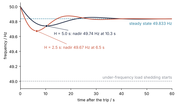
Afterwards you can simulate the grid frequency after a plant trips with solve_ivp and read off the nadir and the rate of change of frequency for any inertia.
- Field
- Engineering, Physics
- Libraries
matplotlib 3.11.2numpy 2.4.3scipy 1.18.1
py-grid-frequency.ipynb, executed with the versions above. The download needs a free account
Run it yourself. In a terminal, this installs exactly the versions above:
pip install numpy==2.4.3 scipy==1.18.1 matplotlib==3.11.2 jupyterlabThe problem
A power plant trips, and the grid frequency falls until the other plants' governors raise their output, a response called primary control. The rotating mass sets how fast it falls, and wind and solar behind inverters add none. You want the rate of change of frequency (RoCoF), the nadir (the minimum), and its margin to 49.0 Hz, continental Europe's load-shedding threshold.
The swing equation (Newton's law for the rotating masses) and a governor lagging by \(T_g\) seconds read
with \(\Delta f\) the frequency deviation as a fraction of nominal \(f_0\), and the lost generation \(\Delta P_\text{loss}\) and extra governor power \(\Delta P_m\) as fractions of system load. \(H\) is the stored kinetic energy over the system load, in seconds, \(D\) the load lost per unit of \(\Delta f\), and \(R\) the droop: the frequency drop over the governor power it calls up. The example halves \(H\) from 5 s to 2.5 s, integrated with solve_ivp. Swap in your own grid.
The code
import numpy as np
import matplotlib.pyplot as plt
from scipy.integrate import solve_ivp

# ---- constants: replace these with your own grid
f0 = 50.0                  # nominal frequency, Hz
dP_loss = 0.01             # lost generation, per unit: the 3,000 MW reference incident on a 300 GW base
D = 0.5                    # load damping, per unit: 1 % of load per Hz
R = 0.4                    # system droop, per unit; 1/R = 2.5: 3,000 MW of primary control at 200 mHz
T_g = 8.0                  # governor and turbine lag, s
inertias = [5.0, 2.5]      # inertia constant H, s: today and halved
t_end = 60.0               # s after the trip
f_shed = 49.0              # Hz, under-frequency load shedding starts

# ---- model: state y = [frequency deviation, extra governor power], both per unit
def rhs(t, y, H):
    df, dPm = y
    return [(dPm - dP_loss - D * df) / (2 * H), (-dPm - df / R) / T_g]

def nadir(t, y, H):
    return rhs(t, y, H)[0]
nadir.direction = 1        # slope crosses zero from falling to rising: a trough

# ---- integrate
t = np.linspace(0, t_end, 1201)
f_ss = f0 * (1 - dP_loss / (D + 1 / R))
results = []
for H in inertias:
    sol = solve_ivp(rhs, (0, t_end), [0.0, 0.0], args=(H,), events=nadir,
                    dense_output=True, rtol=1e-8, atol=1e-10)
    rocof = rhs(0, [0.0, 0.0], H)[0] * f0
    t_nadir = sol.t_events[0][0]                 # the first trough is the deepest
    f_nadir = f0 * (1 + sol.y_events[0][0][0])
    results.append((H, rocof, t_nadir, f_nadir, len(sol.t_events[0]), f0 * (1 + sol.sol(t)[0])))

# ---- report and plot
print(" H / s   RoCoF / (Hz/s)   nadir / Hz   at / s   troughs   steady / Hz   margin to 49.0 / Hz")
for H, rocof, t_n, f_n, troughs, f in results:
    print(f"{H:6.1f}   {rocof:14.3f}   {f_n:10.3f}   {t_n:6.2f}   {troughs:7d}   {f_ss:11.3f}   {f_n - f_shed:19.3f}")

fig, ax = plt.subplots(figsize=(7, 4), dpi=110)
ax.axhline(f_ss, color="#2a7f9e", lw=1, ls="--")
ax.axhline(f_shed, color="#8a8f98", lw=1, ls="--")
ax.text(t_end, f_ss - 0.03, f"steady state {f_ss:.3f} Hz", color="#2a7f9e", ha="right", va="top")
ax.text(t_end, f_shed + 0.02, "under-frequency load shedding starts", color="#8a8f98", ha="right", va="bottom")
for (H, _, t_n, f_n, _, f), color, dy in zip(results, ["#1f2a44", "#c8553d"], [-0.12, -0.24]):
    ax.plot(t, f, color=color, lw=1.8)
    ax.plot(t_n, f_n, "o", color=color, ms=6, mec="white", zorder=3)
    ax.annotate(f"H = {H:.1f} s: nadir {f_n:.2f} Hz at {t_n:.1f} s", (t_n, f_n), (t_n + 3, f_n + dy), color=color,
                arrowprops=dict(arrowstyle="-", color=color, lw=0.8))
ax.set(xlim=(0, t_end), ylim=(48.9, 50.05), xlabel="time after the trip / s", ylabel="frequency / Hz")
ax.spines[["top", "right"]].set_visible(False)
plt.show()
 H / s   RoCoF / (Hz/s)   nadir / Hz   at / s   troughs   steady / Hz   margin to 49.0 / Hz
   5.0           -0.050       49.738    10.33         2        49.833                 0.738
   2.5           -0.100       49.673     6.49         3        49.833                 0.673
The knobs
\(H\) sets the initial slope and the pace of everything after it. At the trip the governors have not moved yet, so only the inertia answers and the RoCoF is \(\Delta P_\text{loss} f_0 / 2H\): −0.050 Hz/s for 5 s, −0.100 Hz/s for 2.5 s. \(R\) and \(D\) set where the frequency settles. Setting both derivatives to zero gives \(\Delta P_m = -\Delta f / R\) from the governor, and \(\Delta f_\text{ss} = -\Delta P_\text{loss} / (D + 1/R)\) from the swing equation. \(H\) does not appear in it, which is why both rows print the same 49.833 Hz. The nadir depends on all four constants, because inertia buys time for a governor that lags by \(T_g\): with half the inertia the frequency falls to 49.673 Hz instead of 49.738 Hz, 65 mHz lower and about 4 s earlier. For your own grid, divide every power by the load base and every frequency by \(f_0\), so a rate per hertz is multiplied by \(f_0\). A 3,000 MW loss on 300 GW is 0.01, load that drops by 1 % per hertz gives \(D = 0.01 \times 50 = 0.5\), and 3,000 MW of primary control deployed at 200 mHz gives \(1/R = 0.01 / 0.004 = 2.5\). That \(R = 0.4\) looks weak next to the 5 % droop of a single unit, which reaches its full rating at a 5 % frequency drop. It is meant to: only part of the fleet provides primary control, and the system's \(R\) is measured on the whole load. With 0.05 for the whole system, \(1/R\) would be 20 instead of 2.5, and the steady deviation would shrink from 167 mHz to 24 mHz.
The model is one bus with one aggregated machine, and linear: no grid topology, no governor deadband, no RoCoF protection, no fast frequency response from inverters and batteries. The margins of 0.738 Hz and 0.673 Hz hold for this loss and these constants only. Do not scale the loss up to find the largest one the grid survives. Primary control in continental Europe is dimensioned for the reference incident and runs out beyond it, which a linear model does not know. For a larger loss, replace dPm in the first entry of the list that rhs returns by min(dPm, reserve), with the available reserve in per unit; the model turns nonlinear, and the margin means something for that loss.
Pitfalls
An event on the frequency instead of its slope. An event that returns \(\Delta f\) fires once, at the trip, where \(\Delta f\) starts from zero, and never again, because the frequency stays below 50 Hz for the whole minute. One that returns \(\Delta f\) minus a guessed threshold fires on the way down, not at the bottom. The nadir is where the slope vanishes, so the event returns the first component of rhs. Keep direction = 1: without it the event also fires at every peak of the overshoot. Keep the first event, too. The recovery oscillates, more with half the inertia, and the troughs column counts two within 60 s for \(H\) = 5 s and three for 2.5 s. Only the first is the nadir.
A trip inside the integration interval. To show the flat 50 Hz before the trip, you start at \(t = -5\) s and switch the loss on with if t > 0 inside rhs. The curve still looks right, but the first event now sits at \(-5\) s and reports 50 Hz as the nadir. Before the trip the slope is exactly zero, and the event fires at nearly every step of the flat start; at the switch the solver then shrinks its steps to fractions of a millisecond to get past the kink. Start at the trip, as the code does, or integrate the flat part separately and attach the event only to the run that starts at the trip.
Hertz in a per-unit equation. Keep \(\Delta f\) in hertz while \(H\) is in seconds and \(D\) and \(R\) are in per unit, and the damping and governor terms come out 50 times too strong while the RoCoF comes out 50 times too small. The nadir then sits a few millihertz below 50 Hz and looks like good news. Keep the state in per unit and multiply by \(f_0\) only for the report and the plot, as the code does, and write the base of \(\Delta P_\text{loss}\) and \(D\) next to their values.