The Lane-Emden equation with solve_ivp: polytropes and the Chandrasekhar mass

The problem

A polytrope is a star whose pressure depends on its density alone, \(P = K\rho^{1+1/n}\). In hydrostatic equilibrium the pressure gradient holds each shell up against the gravity of the mass inside, and with the polytrope law this balance is the Lane-Emden equation

for the density \(\rho = \rho_c\theta^n\) at radius \(r = \alpha\xi\), with

You want the surface, the first zero \(\xi_1\) of \(\theta\), so that \(R = \alpha\xi_1\); the mass constant \(\omega_n = -\xi_1^2\,\theta'(\xi_1)\); and the density profile. With closed forms only for \(n\) = 0, 1, and 5, the example integrates \(n\) = 0 to 4.5 with solve_ivp and turns \(n = 3\) into the Chandrasekhar mass of a white dwarf. Swap in your own indices.

The code

Copy

import numpy as np
import matplotlib.pyplot as plt
from scipy.integrate import solve_ivp
from scipy.constants import hbar, c, G, m_u

# ---- constants: replace the indices and mu_e with your own
indices = [0, 0.5, 1, 1.5, 2, 2.5, 3, 3.5, 4, 4.5]   # polytropic index n, below 5
shown = [0, 1, 1.5, 3, 4, 4.5]                      # the profiles in the figure
mu_e = 2.0                                          # nucleon masses per electron: carbon and oxygen
M_sun = 1.98841e30                                  # kg
xi0, xi_max = 1e-6, 1e3                             # start off the singular center; end past any surface

# ---- model: y = [theta, dtheta/dxi]
def lane_emden(xi, y, n):
    theta, dtheta = y
    return [dtheta, -np.maximum(theta, 0.0) ** n - 2 * dtheta / xi]   # no density outside the star

def surface(xi, y, n):
    return y[0]
surface.terminal = True
surface.direction = -1

def solve(n, rtol=1e-10, atol=1e-12):
    y0 = [1 - xi0**2 / 6 + n * xi0**4 / 120, -xi0 / 3 + n * xi0**3 / 30]   # series about the center
    return solve_ivp(lane_emden, (xi0, xi_max), y0, args=(n,), events=surface,
                     dense_output=True, rtol=rtol, atol=atol)

# ---- integrate
results = {}
for n in indices:
    sol = solve(n)
    xi1 = sol.t_events[0][0]
    omega = -xi1**2 * sol.y_events[0][0][1]
    results[n] = (sol, xi1, omega)

# ---- report and plot
print("   n        xi_1    omega_n")
for n, (sol, xi1, omega) in results.items():
    print(f"{n:4.1f}  {xi1:10.5f}  {omega:9.5f}")
print(f"xi_1 - sqrt(6) for n = 0: {results[0][1] - np.sqrt(6):.1e}")
print(f"xi_1 - pi      for n = 1: {results[1][1] - np.pi:.1e}")
M_ch = np.sqrt(3 * np.pi) / 2 * results[3][2] * (hbar * c / G) ** 1.5 / m_u**2 / M_sun
print(f"M_Ch = {M_ch:.3f} / mu_e^2 M_sun = {M_ch / mu_e**2:.3f} M_sun for mu_e = {mu_e:.2f}, "
      f"{M_ch / (56 / 26) ** 2:.3f} M_sun for iron")
print("rho / rho_c at r = R/2:", ", ".join(f"{np.maximum(results[n][0].sol(results[n][1] / 2)[0], 0) ** n:.2g} (n = {n:g})" for n in shown))

fig, ax = plt.subplots(figsize=(7, 4), dpi=110)
x = np.linspace(0, 1, 400)                          # r / R
for k, n in enumerate(shown):
    sol, xi1, _ = results[n]
    rho = np.maximum(sol.sol(np.maximum(x * xi1, xi0))[0], 0.0) ** n
    color = plt.cm.cividis(0.75 * n / max(shown))      # the light top of cividis is cut: unreadable on white
    ax.plot(x, rho, color=color, lw=1.8)
    ax.text(0.70, 0.90 - 0.08 * k, f"n = {n:g},  ξ₁ = {xi1:.2f}", color=color, va="center", weight="bold")
ax.set(xlim=(0, 1), ylim=(0, 1.08), xlabel="r / R", ylabel="ρ / ρ$_c$")
ax.spines[["top", "right"]].set_visible(False)
plt.show()

   n        xi_1    omega_n
 0.0     2.44949    4.89898
 0.5     2.75270    3.78865
 1.0     3.14159    3.14159
 1.5     3.65375    2.71406
 2.0     4.35287    2.41105
 2.5     5.35528    2.18720
 3.0     6.89685    2.01824
 3.5     9.53581    1.89056
 4.0    14.97155    1.79723
 4.5    31.83646    1.73780
xi_1 - sqrt(6) for n = 0: 8.9e-16
xi_1 - pi      for n = 1: 1.6e-11
M_Ch = 5.825 / mu_e^2 M_sun = 1.456 M_sun for mu_e = 2.00, 1.256 M_sun for iron
rho / rho_c at r = R/2: 1 (n = 0), 0.64 (n = 1), 0.42 (n = 1.5), 0.023 (n = 3), 0.00021 (n = 4), 2.1e-06 (n = 4.5)

The knobs

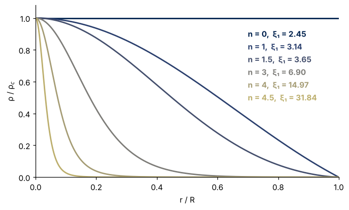
The center is singular, because \(2\theta'/\xi\) is zero over zero there, so the code starts at xi0 \(= 10^{-6}\) with the series you get by putting \(\theta = 1 + a\xi^2 + b\xi^4\) into the equation, \(a = -1/6\) and \(b = n/120\), and its derivative for \(\theta'\). With the series the start hardly matters (Pitfalls). The solution begins at xi0, so the plot evaluates it at np.maximum(x * xi1, xi0). rtol and atol set how many digits of \(\xi_1\) are right, and the defaults already get the third one wrong. xi_max must lie past the surface: \(\xi_1\) grows from 2.45 at \(n = 0\) to 14.97 at \(n = 4\) and 31.84 at \(n = 4.5\). For \(n \ge 5\) there is no surface, as the closed form \(\theta = (1 + \xi^2/3)^{-1/2}\) at \(n = 5\) shows, and t_events[0][0] raises an IndexError. mu_e is the number of nucleon masses per electron, so that \(\rho = \mu_e m_u n_e\) with \(m_u\) the atomic mass constant and \(n_e\) the number of electrons per volume: 2 for carbon and oxygen, giving 1.456 M☉, and 56/26 for iron, giving 1.256 M☉.

Multiplied by \(\xi^2\), the equation reads \((\xi^2\theta')' = -\xi^2\theta^n\), so integrating it once from the center gives \(\int_0^{\xi_1}\xi^2\theta^n\,d\xi = -\xi_1^2\,\theta'(\xi_1) = \omega_n\), and that integral is the mass in units of \(4\pi\alpha^3\rho_c\):

The power of \(\rho_c\) vanishes at \(n = 3\): a star with \(n = 3\) and a given \(K\) has one mass, whatever its central density. A white dwarf is held up by the pressure of degenerate electrons, and once they are ultra-relativistic that pressure is a polytrope with \(n = 3\) and

Put this \(K\) into the mass and you get the line the code evaluates,

That is a limit, not the mass of every white dwarf. A lighter one has slow electrons, so \(n = 1.5\) and \(M \propto \rho_c^{1/2}\): more mass needs a higher central density. As that density grows, the electrons turn ultra-relativistic and the mass approaches \(M_\text{Ch}\) from below, for an ideal electron gas. In the figure, the higher \(n\), the more the mass gathers at the center: at half the radius the density is 64 % of its central value for \(n = 1\) but 2.3 % for \(n = 3\). The lines are colored by \(n\) with the cividis colormap.

Pitfalls

Starting at the center. Integrate from (0, xi_max) and the call never returns: at \(\xi = 0\) the slope is zero over zero, and NumPy warns. The cell shows the warning, then starts at \(10^{-2}\), once with \(\theta = 1\), \(\theta' = 0\) and once with the series, because at \(10^{-6}\) the two agree to the ninth decimal:

import warnings

with warnings.catch_warnings(record=True) as caught:
    warnings.simplefilter("always")
    print("right-hand side at the center:", [float(v) for v in lane_emden(0.0, np.array([1.0, 0.0]), 3)])
print(f"{caught[0].category.__name__}: {caught[0].message}")
for label, y0 in [("theta = 1, theta' = 0", [1.0, 0.0]), ("series", [1 - 1e-4 / 6 + 3e-8 / 120, -1e-2 / 3 + 3e-6 / 30])]:
    sol = solve_ivp(lane_emden, (1e-2, xi_max), y0, args=(3,), events=surface, rtol=1e-10, atol=1e-12)
    print(f"start at xi = 1e-2, {label:22s}: xi_1 = {sol.t_events[0][0]:.5f}")

right-hand side at the center: [0.0, nan]
RuntimeWarning: invalid value encountered in scalar divide
start at xi = 1e-2, theta = 1, theta' = 0 : xi_1 = 6.89650
start at xi = 1e-2, series                : xi_1 = 6.89685

The first step size solve_ivp estimates from that slope is NaN as well, and since every comparison with NaN is false, the step is never accepted and never judged too small to give up on. Without the series the surface moves from 6.89685 to 6.89650, in the fifth digit. Start at \(10^{-6}\) with the series, as the code does.

NaN past the surface for a non-integer n. Write theta ** n without the clip, and \(n = 1.5\) fails with the terminal event in place:

def lane_emden_unclipped(xi, y, n):
    theta, dtheta = y
    return [dtheta, -theta ** n - 2 * dtheta / xi]

n = 1.5
y0 = [1 - xi0**2 / 6 + n * xi0**4 / 120, -xi0 / 3 + n * xi0**3 / 30]
with warnings.catch_warnings(record=True) as caught:
    warnings.simplefilter("always")
    sol = solve_ivp(lane_emden_unclipped, (xi0, xi_max), y0, args=(n,), events=surface, rtol=1e-10, atol=1e-12)
print(f"{caught[0].category.__name__}: {caught[0].message}")
print(f"status {sol.status}: {sol.message}")
print(f"stopped at xi = {sol.t[-1]:.5f}, t_events = {sol.t_events[0]}")

RuntimeWarning: invalid value encountered in scalar power
status -1: Required step size is less than spacing between numbers.
stopped at xi = 3.65375, t_events = []

solve_ivp looks for an event only after finishing a step, by a sign change of the event function between the step's ends, and then finds the zero with the solution in between. To take a step, RK45 evaluates the right-hand side at trial points ahead of the current one, and near the surface those lie where \(\theta < 0\) and \(\theta^{1.5}\) is NaN. A NaN error estimate fails the accuracy test, so the solver rejects the step and shrinks it to the smallest it allows, then gives up at \(\xi_1\) to five decimals, with no event recorded. A terminal event does not stop the right-hand side from being called past the zero, so it must be defined there: clip with np.maximum(theta, 0.0) ** n, no density outside the star. Do not use np.abs, which integrates a mirrored star beyond the surface and hides the mistake when the event is missing.

The default tolerances. Leave out rtol and atol, and solve_ivp uses rtol=1e-3, atol=1e-6:

sol = solve(3, rtol=1e-3, atol=1e-6)
xi1 = sol.t_events[0][0]
print(f"default tolerances: xi_1 = {xi1:.5f}, omega_3 = {-xi1**2 * sol.y_events[0][0][1]:.5f}")

default tolerances: xi_1 = 6.90833, omega_3 = 2.01663

The surface is off in the third digit, 6.90833 against 6.89685, and \(\omega_3\), 2.01663 against 2.01824, passes its error into the Chandrasekhar mass. Keep the tolerances of the code, and to check that an answer has converged, run ten times tighter.