Draw a phase portrait of a two-variable ODE system

Afterwards you can integrate a two-variable ODE system with solve_ivp, find its fixed points, and draw its phase portrait over a direction field.

Topic: Ordinary differential equations
Field: Cross-disciplinary
Libraries: matplotlib 3.11.2, numpy 2.5.3, scipy 1.18.1
Prerequisites: none beyond Python basics
Notebook: Download py-phase-portrait.ipynb, executed with the versions above

The problem

You have a two-variable system of first-order ODEs and want its phase portrait: the plane of the two variables, with time eliminated. An arrow at each grid point shows where a state there moves: the direction field. Over it go trajectories, each the succession of states the system passes through in time from one start, integrated with solve_ivp. Fixed points, or steady states, are where both derivatives vanish.

The example is the Lotka-Volterra predator-prey model, \(\dot x = \alpha x - \beta xy\) and \(\dot y = \delta xy - \gamma y\), with prey \(x\) and predators \(y\) in thousands, \(t\) in years, and rates \(\alpha, \beta, \gamma, \delta\). Swap in your own right-hand side, parameters, window, and starting points.

The code

import numpy as np
import matplotlib.pyplot as plt
from scipy.integrate import solve_ivp
from scipy.optimize import root

# ---- system: replace f, its parameters, the window, and the starts with your own
alpha, gamma = 1.0, 0.6        # prey growth, predator death; per year
beta, delta = 2.0, 0.2         # predation, predator gain from prey; per thousand per year

def f(t, z):                   # the form solve_ivp wants: time t first, then the state z = [x, y]
    x, y = z                   # prey, predators, in thousands
    return [alpha * x - beta * x * y, delta * x * y - gamma * y]   # NumPy arithmetic: works on grids

xlim, ylim = (0, 9), (0, 1.5)  # the window: what the figure shows and where root looks
starts = [(3, 0.65), (3, 0.875), (3, 1.125), (3, 1.375)]

# ---- direction field: f on a grid
X, Y = np.meshgrid(np.linspace(*xlim, 21), np.linspace(*ylim, 15))
U, V = f(0, [X, Y])                            # the whole grid in one call; t does not enter f
speed = np.hypot(U, V)
norm = np.where(speed > 0, speed, 1.0)         # a node on a fixed point keeps a zero arrow, no 0 / 0
u, v = U / norm, V / norm                      # unit length: raw lengths would hide the slow regions

# ---- fixed points (steady states): root finds one zero of f per guess, so try a 5 x 5 grid
fixed = []
gx, gy = np.meshgrid(np.linspace(*xlim, 5), np.linspace(*ylim, 5))
for guess in zip(gx.ravel(), gy.ravel()):
    r = root(lambda z: f(0, z), guess)         # root wants a function of the state only
    if not r.success:                          # a failed guess is reported here, not as a warning
        continue
    p = np.round(r.x, 6) + 0.0                 # -1e-15 would print -0.000; + 0.0 drops the sign
    inside = xlim[0] <= p[0] <= xlim[1] and ylim[0] <= p[1] <= ylim[1]   # else drawn off the axes
    if inside and not any(np.allclose(p, q) for q in fixed):   # many guesses find the same point
        fixed.append(p)

# ---- trajectories
t = np.linspace(0, 12, 1200)                   # t_eval: when to report the state, in years
trajectories = [solve_ivp(f, (0, 12), z0, t_eval=t,   # t_span (0, 12): the interval integrated
                          rtol=1e-8, atol=1e-10).y    # tighter than the loose defaults
                for z0 in starts]                     # .y: rows x and y, one column per time
leaving = sum(np.any((x < xlim[0]) | (x > xlim[1]) | (y < ylim[0]) | (y > ylim[1]))
              for x, y in trajectories)               # these run past the frame, which clips them

# ---- report and plot
print("fixed points:", "  ".join(f"({x:.3f}, {y:.3f})" for x, y in fixed))
print(f"arrow speeds on the grid: {speed[speed > 0].min():.3g} to {speed.max():.3g}")
print(f"trajectories leaving the window: {leaving} of {len(trajectories)}")

fig, ax = plt.subplots(figsize=(7, 4), dpi=110)
ax.quiver(X, Y, u, v, color="#8a8f98", angles="xy", pivot="middle", width=0.003)  # direction field
for (x, y), (x0, y0) in zip(trajectories, starts):
    ax.plot(x, y, color="#c8553d", lw=1.6)
    ax.plot(x0, y0, "o", color="#c8553d", ms=4)
for x, y in fixed:                             # clip_on=False: the origin sits on the corner
    ax.plot(x, y, "o", color="#1f2a44", ms=7, clip_on=False, zorder=3)
# limits turn autoscaling off, before or after plotting; it would fit the trajectory that leaves
ax.set(xlim=xlim, ylim=ylim, xlabel="prey / thousands", ylabel="predators / thousands")
ax.spines[["top", "right"]].set_visible(False)
plt.show()

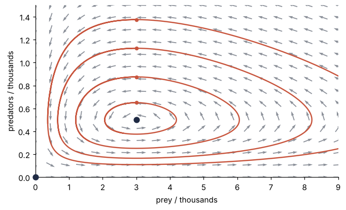
fixed points: (0.000, 0.000)  (3.000, 0.500)
arrow speeds on the grid: 0.0643 to 18.1
trajectories leaving the window: 1 of 4

The knobs

The 21 × 15 grid puts 21 arrows across the figure, enough to follow the flow. angles="xy" points each arrow from \((x, y)\) toward \((x + u, y + v)\) in data coordinates. Matplotlib's default, "uv", sets the angle on the screen, which is wrong for a phase portrait: with prey up to 9 thousand and predators up to 1.5 thousand, the arrows lie almost flat and cross the trajectories. The 5 × 5 guesses span the window, and fixed points outside it are dropped, so choose it to contain the ones you care about, with a margin. A fixed point inside that no guess converges to is missed until you add guesses. The starts, the small dots, sit on a vertical line through the fixed point at \((3, 0.5)\), so the closed trajectories nest. For a system that settles, start along the edge of the window and near each fixed point. t_span, not t, is the setting to lengthen. For closed trajectories it must let the widest one close, as 12 years does here, and for a system that settles it must let the slowest one arrive. A trajectory that ends in midair means the span stopped short. Move the end of t with it: with t unchanged, a longer span integrates further and still draws nothing past 12 years. The 1200 points can stay, since they only set how smoothly a trajectory is drawn. For the tolerances, see the accuracy step of the solve_ivp tutorial.

Each arrow gives the direction of motion at its midpoint and nothing about speed, because all have one length. Color brings the speed back: ax.quiver(X, Y, u, v, speed, cmap="cividis", ...). The first printed line agrees with the equations. \((0, 0)\) is extinction, visible in f because each derivative carries a factor of its own variable, and \((3, 0.5)\) is \((\gamma/\delta, \alpha/\beta)\), which checks root against the hand solution. A fixed-point marker says where f vanishes, not whether nearby states approach it; the trajectories answer that. Here they circle \((3, 0.5)\) without reaching it, and near the origin states arrive along the predator axis and leave along the prey axis. The picture assumes f does not depend on \(t\). For a driven system the arrows change with time and trajectories cross, and the tool there is a Poincaré section, named in the variations of the solve_ivp tutorial.

Pitfalls

Arrows scaled by speed. Hand U, V to quiver instead of u, v, and the arrows around both fixed points shrink to dots while the upper right fills with long arrows that run into each other. The second printed line says why: speeds from 0.0643 to 18.1 thousand per year on this grid, a factor of 281. quiver scales every arrow by one common factor, chosen from the average arrow length, so arrows far below the average vanish and arrows far above it overlap. The slow regions are the ones you drew the portrait for, because every fixed point sits in one. Normalize as the code does, guard included. Without the guard, the grid node at the origin divides zero by zero and NumPy prints a RuntimeWarning.

Trajectories that run past the window. The last printed line says 1 of 4: the outermost trajectory runs off the right edge and comes back. Leave the limits out of ax.set, and autoscaling widens the axes to fit the trajectory while the arrows stop short of the new edge. Without limits, a trajectory that runs away to \(10^6\) squeezes the portrait against one edge. For such a system, also stop the integration with an event function box(t, z), positive inside a box larger than the window and negative outside. solve_ivp detects an event only where the function changes sign over a step, and a distance to the edge never does. Set box.terminal = True and pass events=box: solve_ivp then stops at the edge. The solve_ivp tutorial covers events in full.

Too many arrows. On a fine grid, say 60 × 60, the arrows shrink to specks and no direction can be read. Use ax.streamplot(X, Y, U, V, color="#8a8f98", density=1.5) instead, with the raw components; density sets how closely its lines pack. It needs an evenly spaced grid, like the one in the code. Its lines come from its own integrator on the field interpolated between grid nodes, not on f, so they show the flow but do not solve your equations to any tolerance. The trajectories on top therefore still come from solve_ivp.