SymPy from the ground up: where the pendulum's 1.74 % comes from

The problem: where does the 1.74 % come from?

The small-angle period of a pendulum is \(T_0 = 2\pi\sqrt{L/g}\), 2.006 s for a 1 m pendulum. Released at 30°, the same pendulum takes 1.74 % longer, and tables of corrections say that the excess grows as the square of the amplitude. With SymPy, Python's computer algebra system, you can derive that correction yourself instead of looking it up:

The road goes from the energy of the pendulum to its angular velocity, from there to the period as an integral, through a change of variables that makes the integral expandable, and to a series integrated term by term. At the end you solve the series for the amplitude at which the correction reaches 1 % and turn it into a NumPy function. solve_ivp from the ground up measured the period by integrating the motion, and Numerical integration with scipy.integrate computed it with quad. This tutorial finds the formula behind their numbers.

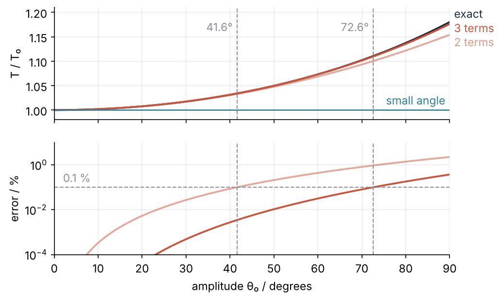
This is where we end up. The series come from SymPy, the exact curve from quad, and the lower panel shows how far each truncation carries before it is off by more than a tenth of a percent.

Setup

import numpy as np
import sympy as sp
import matplotlib.pyplot as plt
from scipy.integrate import quad

plt.rcParams.update({
    "figure.figsize": (7, 3.6), "figure.dpi": 110,
    "axes.spines.top": False, "axes.spines.right": False,
    "axes.grid": True, "grid.alpha": 0.25,
    "font.size": 11, "lines.linewidth": 1.8,
})
INK, ACCENT, SECOND, MUTED = "#1f2a44", "#c8553d", "#2a7f9e", "#8a8f98"

print(f"SymPy {sp.__version__}")

SymPy 1.14.0

Step 1: Build expressions from symbols

A SymPy symbol is a name that stays a name: arithmetic on it builds an expression instead of a number. We need five: \(\theta\) the angle, \(\theta_0\) the amplitude, \(\dot\theta = d\theta/dt\) the angular velocity (hence theta_dot, not omega, which would read as the frequency \(\sqrt{g/L}\)), \(L\) the length, and \(g\) gravity. The energy per unit mass is \(E = \tfrac12 L^2\dot\theta^2 + gL(1 - \cos\theta)\):

theta, theta0, theta_dot, L, g = sp.symbols("theta theta0 theta_dot L g", positive=True)

E = sp.Rational(1, 2) * L**2 * theta_dot**2 + g * L * (1 - sp.cos(theta))
print(E)

L**2*theta_dot**2/2 + L*g*(1 - cos(theta))

print shows a result as one line of plain text that you can copy back into code, and every result below is shown that way. sp.cos is SymPy's cosine, and sp.Rational(1, 2) is an exact half. positive=True tells SymPy which signs and roots are possible, and it decides what solve returns in Steps 2 and 5.

At the turning point the bob is at \(\theta_0\) and at rest. subs replaces symbols, several at once from a dictionary, and evalf turns an exact result into digits:

E0 = E.subs({theta: theta0, theta_dot: 0})
E0_30 = E0.subs(theta0, sp.pi / 6)
print(E0)
print(E0_30)
print(E0_30.subs({L: 1, g: 9.81}).evalf(), "J/kg")

L*g*(1 - cos(theta0))
L*g*(1 - sqrt(3)/2)
1.31429078887466 J/kg

SymPy keeps \(1 - \sqrt3/2\) exact until you ask for digits. For a 1 m pendulum at 30° that is 1.314 J/kg, against 9.81 J/kg for a release at 90°.

Step 2: Differentiate and solve: from the energy to the period integral

Before the period, two checks that \(E\) describes the pendulum you know. Its time derivative must give the equation of motion that solve_ivp integrates, and the series of \(\sin\theta\) must give back the harmonic oscillator, whose period is the \(T_0\) that every result below is measured against. To SymPy, theta is a plain symbol with no time in it, so its derivative with respect to \(t\) is zero. Make \(\theta\) a function of \(t\) and put it in place of both symbols:

t = sp.symbols("t")
th = sp.Function("theta")(t)
E_t = E.subs({theta: th, theta_dot: th.diff(t)})
dE_dt = sp.diff(E_t, t)
print(E_t)
print(dE_dt)

L**2*Derivative(theta(t), t)**2/2 + L*g*(1 - cos(theta(t)))
L**2*Derivative(theta(t), t)*Derivative(theta(t), (t, 2)) + L*g*sin(theta(t))*Derivative(theta(t), t)

SymPy does not know that energy is conserved. The physics sets dE_dt to zero, and solve takes the second derivative as its unknown just as it would take a symbol. series(expr, x, x0, n) expands around \(x_0\), here 0, and stops before the power \(x^n\):

print(sp.solve(sp.Eq(dE_dt, 0), th.diff(t, 2)))
print(sp.series(sp.sin(theta), theta, 0, 4))

[-g*sin(theta(t))/L]
theta - theta**3/6 + O(theta**4)

That is \(\ddot\theta = -(g/L)\sin\theta\). Both terms of dE_dt carry \(\dot\theta\), and solve divided it out, assuming the pendulum is moving. Without Eq, as in much other code, solve(expr, x) solves expr = 0. Drop the cube of the sine and you have the harmonic oscillator.

Now solve energy conservation, \(E = E_0\), for the angular velocity. solve returns a list, here of one root:

T0 = 2 * sp.pi * sp.sqrt(L / g)
theta_dot_expr = sp.solve(sp.Eq(E, E0), theta_dot)[0]
print(theta_dot_expr)

sqrt(2)*sqrt(g)*sqrt(cos(theta) - cos(theta0))/sqrt(L)

positive=True excluded the negative root. A quarter swing from \(0\) to \(\theta_0\) takes \(T/4\), so \(T = 4\int_0^{\theta_0} d\theta/\dot\theta\). Ask SymPy for it:

attempt = sp.integrate(1 / theta_dot_expr, (theta, 0, theta0))
print(attempt)
print((1 / theta_dot_expr).subs(theta, theta0))

sqrt(2)*sqrt(L)*Integral(1/sqrt(cos(theta) - cos(theta0)), (theta, 0, theta0))/(2*sqrt(g))
zoo

SymPy pulled out the constants and handed the rest back as an unevaluated Integral, which is how integrate says it failed. The integrand at \(\theta = \theta_0\) is zoo, SymPy's complex infinity: the singular endpoint that quad handled in the quad tutorial. Nor can you expand it in \(\theta_0\) as it stands: a series around \(\theta_0 = 0\) at fixed \(\theta\) passes through \(\theta_0 < \theta\), where the square root is imaginary.

Step 3: Change variables, and choose how SymPy rewrites

The standard way out is the substitution \(\sin(\theta/2) = k\sin\varphi\) with \(k = \sin(\theta_0/2)\). As \(\theta\) runs from 0 to \(\theta_0\), \(\varphi\) runs from 0 to \(\pi/2\), so \(\theta_0\) leaves the limits and lives only in \(k\). The integral then needs three pieces written in \(\varphi\): the factor \(d\theta/d\varphi\) in \(d\theta = (d\theta/d\varphi)\,d\varphi\), and \(\cos\theta\) and \(\cos\theta_0\), the only places where the angles enter \(\dot\theta\). diff gives the factor. expand_trig gives the cosines: it applies the sum and multiple-angle identities, so that cos(2*phi) becomes 2*cos(phi)**2 - 1, and here it takes the asin out of the cosine:

k, phi = sp.symbols("k phi", positive=True)
theta_of_phi = 2 * sp.asin(k * sp.sin(phi))
dtheta_dphi = sp.diff(theta_of_phi, phi)
cos_theta = sp.expand_trig(sp.cos(theta_of_phi))
cos_theta0 = sp.expand_trig(sp.cos(2 * sp.asin(k)))
print(dtheta_dphi)
print(cos_theta)
print(cos_theta0)

2*k*cos(phi)/sqrt(-k**2*sin(phi)**2 + 1)
-2*k**2*sin(phi)**2 + 1
1 - 2*k**2

Put the two cosines into the angular velocity from Step 2 and simplify. The result, theta_dot_phi, is \(\dot\theta\) written in \(\varphi\):

theta_dot_phi = sp.simplify(theta_dot_expr.subs({sp.cos(theta): cos_theta, sp.cos(theta0): cos_theta0}))
print(theta_dot_phi)

2*sqrt(g)*k*Abs(cos(phi))/sqrt(L)

The Abs is there because SymPy does not know that \(\varphi\) stays between 0 and \(\pi/2\), where the cosine is positive. We know it, and no symbol property says it, so we replace the absolute value by hand:

theta_dot_phi = theta_dot_phi.subs(sp.Abs(sp.cos(phi)), sp.cos(phi))
integrand = sp.simplify(dtheta_dphi / theta_dot_phi)
T = 4 * sp.Integral(integrand, (phi, 0, sp.pi / 2))
print(T)

4*Integral(sqrt(L)/(sqrt(g)*sqrt(-k**2*sin(phi)**2 + 1)), (phi, 0, pi/2))

SymPy carried every prefactor, and the period is

No infinity left, and \(k\) sits where a series can reach it.

Two kinds of rewrite tool did the work. expand_trig is targeted: it does one predictable thing, and expand, factor, and trigsimp are of the same kind. simplify is a heuristic that tries many rewrites and keeps the shortest result, and it promises no particular form. When you know the form you want, call the targeted tool. When you only want something shorter, call simplify.

Step 4: Expand in a series and integrate term by term

Expand the integrand in powers of \(k\), drop the order term with removeO (integrate would carry an O(k**6) along, but lambdify in Step 6 refuses to turn it into NumPy code), and integrate each term over \(\varphi\):

print(sp.series(integrand, k, 0, 6))
phi_integral = sp.integrate(sp.series(integrand, k, 0, 6).removeO(), (phi, 0, sp.pi / 2))
print(sp.expand(4 * phi_integral / T0))

sqrt(L)/sqrt(g) + sqrt(L)*k**2*sin(phi)**2/(2*sqrt(g)) + 3*sqrt(L)*k**4*sin(phi)**4/(8*sqrt(g)) + O(k**6)
9*k**4/64 + k**2/4 + 1

expand multiplies out and lets the \(\sqrt{L/g}\) cancel; series is the expansion in powers. What is left is \(T/T_0\) in \(k\). Now put in \(k = \sin(\theta_0/2)\) to get ratio, the period ratio as a function of the amplitude, and expand that in \(\theta_0\):

ratio = sp.expand(4 * phi_integral / T0).subs(k, sp.sin(theta0 / 2))
print(sp.series(ratio, theta0, 0, 6))

two = sp.series(ratio, theta0, 0, 4).removeO()
three = sp.series(ratio, theta0, 0, 6).removeO()
print(two)
print(three)
for name, term in [("theta0^2", theta0**2 / 16), ("theta0^4", 11 * theta0**4 / 3072)]:
    print(f"{name} term at 30°: {float(term.subs(theta0, sp.pi / 6)):.5f}")
print(f"T/T0 at 30°, three terms: {float(three.subs(theta0, sp.pi / 6)):.4f}")

1 + theta0**2/16 + 11*theta0**4/3072 + O(theta0**6)
theta0**2/16 + 1
11*theta0**4/3072 + theta0**2/16 + 1
theta0^2 term at 30°: 0.01713
theta0^4 term at 30°: 0.00027
T/T0 at 30°, three terms: 1.0174

two and three are the truncations with two and three terms. At 30° the first correction is 0.01713 and the second 0.00027, about 64 times smaller, and together they give 1.0174: the 1.74 % of the title. The \(k^6\) term we dropped starts at \(\theta_0^6\), so the \(\theta_0^4\) coefficient is complete.

Step 5: Solve for the amplitude of a 1 % correction

At what amplitude is the period 1 % longer than \(T_0\)? With the two-term series:

root_two = sp.solve(sp.Eq(two - 1, sp.Rational(1, 100)), theta0)
print(root_two)
print(sp.deg(root_two[0]), "=", sp.deg(root_two[0]).evalf(4), "degrees")

[2/5]
72/pi = 22.92 degrees

An exact 2/5 rad, the only root because positive=True excludes −2/5. sp.deg converts to degrees and stays exact, \(72/\pi\), until evalf(4) makes it 22.92°, four significant digits. The three-term series gives a quartic in \(\theta_0\):

root_three = sp.solve(sp.Eq(three - 1, sp.Rational(1, 100)), theta0)
print(root_three)
print(sp.deg(root_three[0]).evalf(4), "degrees")

[4*sqrt(-6/11 + sqrt(933)/55)]
22.81 degrees

A nested radical, and 22.81°. The fourth-order term moves the answer by a tenth of a degree. Which of the two is right shows up in Step 6, against the exact period.

Step 6: Turn the series into NumPy functions and compare with quad

lambdify turns a SymPy expression into a plain Python function that works on NumPy arrays:

ratio_two = sp.lambdify(theta0, two, "numpy")
ratio_three = sp.lambdify(theta0, three, "numpy")
print(ratio_two(np.radians([30, 60])), ratio_three(np.radians([30, 60])))

[1.01713473 1.06853892] [1.01740386 1.07284504]

The exact ratio is the integral of Step 2 divided by \(T_0\), where the prefactor \(\sqrt{L/2g}\) that SymPy pulled out, times 4, over \(2\pi\sqrt{L/g}\) leaves \(\sqrt2/\pi\):

quad handles it despite the infinity at the upper end, as the quad tutorial explains. Sweep the amplitude from 0.1° to 90° in steps of 0.1°, 900 calls to quad:

Copy

def exact_ratio(th0):
    val, _ = quad(lambda th: 1 / np.sqrt(np.cos(th) - np.cos(th0)), 0, th0)
    return np.sqrt(2) / np.pi * val

amp = np.round(np.arange(1, 901) * 0.1, 1)          # degrees, rounded so that amp == 30 finds 30°
exact = np.array([exact_ratio(a) for a in np.radians(amp)])
err_two = 100 * np.abs(ratio_two(np.radians(amp)) / exact - 1)      # percent
err_three = 100 * np.abs(ratio_three(np.radians(amp)) / exact - 1)

def good_up_to(err):
    return amp[np.argmax(err > 0.1) - 1]             # last amplitude before 0.1 % is exceeded

lim_two, lim_three = good_up_to(err_two), good_up_to(err_three)

fig, (ax1, ax2) = plt.subplots(2, 1, sharex=True, figsize=(7, 4.4))
ax1.plot(amp, exact, color=INK)
ax1.plot(amp, ratio_three(np.radians(amp)), color=ACCENT)
ax1.plot(amp, ratio_two(np.radians(amp)), color=ACCENT, alpha=0.5)
ax1.axhline(1, color=SECOND, lw=1.2)
ax1.text(89, 1.006, "small angle", color=SECOND, ha="right", va="bottom")
ax1.text(91, exact[-1] + 0.017, "exact", color=INK, va="center")
ax1.text(91, ratio_three(np.pi / 2) - 0.008, "3 terms", color=ACCENT, va="center")
ax1.text(91, ratio_two(np.pi / 2) - 0.015, "2 terms", color=ACCENT, alpha=0.6, va="center")
ax1.set(ylabel="T / T₀", ylim=(0.98, 1.21))
ax2.semilogy(amp, err_three, color=ACCENT)
ax2.semilogy(amp, err_two, color=ACCENT, alpha=0.5)
ax2.axhline(0.1, color=MUTED, lw=1, ls="--")
ax2.text(2, 0.13, "0.1 %", color=MUTED, va="bottom")
for lim in (lim_two, lim_three):
    for ax in (ax1, ax2):
        ax.axvline(lim, color=MUTED, lw=1, ls="--")
    ax1.text(lim - 1, 1.17, f"{lim}°", color=MUTED, ha="right", va="center")
ax2.set(xlabel="amplitude θ₀ / degrees", ylabel="error / %", xlim=(0, 90), ylim=(1e-4, 10))
plt.show()

for a in (30, 60, 90):
    i = np.flatnonzero(amp == a)[0]
    print(f"{a:2d}°  T/T0 = {exact[i]:.4f}   error 2 terms {err_two[i]:.4f} %   3 terms {err_three[i]:.4f} %")
print(f"within 0.1 %: 2 terms up to {lim_two}°, 3 terms up to {lim_three}°")
print(f"exact T/T0 at 2/5 rad: {exact_ratio(0.4):.5f}")
print(f"exact T/T0 at {float(sp.deg(root_three[0])):.2f}°: {exact_ratio(float(root_three[0])):.5f}")

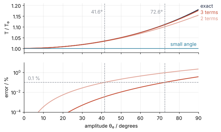
30°  T/T0 = 1.0174   error 2 terms 0.0269 %   3 terms 0.0005 %
60°  T/T0 = 1.0732   error 2 terms 0.4326 %   3 terms 0.0314 %
90°  T/T0 = 1.1803   error 2 terms 2.2136 %   3 terms 0.3667 %
within 0.1 %: 2 terms up to 41.6°, 3 terms up to 72.6°
exact T/T0 at 2/5 rad: 1.01009
exact T/T0 at 22.81°: 1.01000

The third term extends the 0.1 % range from 41.6° to 72.6°. At 90° the two-term series is 2.2 % short and the three-term series 0.37 %. The exact ratio at 2/5 rad is 1.01009, so the two-term answer of Step 5 overshoots the 1 % amplitude by a little. At the three-term answer of 22.81° it is 1.01000: the quartic was the right one to solve. The two-term formula, the one most textbooks print, is good to a tenth of a percent up to about 40°, which covers almost every pendulum anyone times in a lab.

Pitfalls

Python floats where you wanted fractions. Write the coefficient first and Python divides before SymPy sees a symbol:

print(1/16 * theta0**2)
print(sp.solve(sp.Eq(theta0**2 / 16, 0.01), theta0))

0.0625*theta0**2
[0.400000000000000]

The exact 2/5 of Step 5 is gone, and every later step carries 15-digit floats. Put the symbol first (theta0**2/16), or write sp.Rational(1, 16) and sp.Rational(1, 100).

NumPy functions on symbols. np.sin does not know what a symbol is:

try:
    np.sin(theta)
except TypeError as err:
    print("TypeError:", err)

TypeError: loop of ufunc does not support argument 0 of type Symbol which has no callable sin method

The reverse, sp.sin on an array, is just as wrong. Use sp. functions while you derive, and cross over to NumPy once, with lambdify.

Forgetting assumptions. Without positive=True, SymPy has to allow every sign:

x = sp.symbols("x")
print(sp.solve(sp.Eq(x**2 / 16, sp.Rational(1, 100)), x))
print(sp.sqrt(x**2))

[-2/5, 2/5]
sqrt(x**2)

Two roots instead of one, and \(\sqrt{x^2}\) stays as it is, because it equals \(x\) only for \(x \ge 0\). Declare positive=True or real=True whenever it is true. For a range no symbol property can express, replace the Abs by hand as in Step 3.

Variations

• More terms. Expand in \(k\) to O(k**10) and in \(\theta_0\) to O(theta0**8), and the next coefficient appears: 173*theta0**6/737280.
• Name the integral. The integral \(\int_0^{\pi/2} d\varphi/\sqrt{1 - m\sin^2\varphi}\) is, by definition, the complete elliptic integral of the first kind \(K(m)\), with \(m = k^2 = \sin^2(\theta_0/2)\). sp.simplify(T / T0) on the unevaluated integral of Step 3 prints 2*elliptic_k(k**2)/pi, and sp.series(sp.elliptic_k(m), m, 0, 3) gives the series of Step 4 directly. scipy.special.ellipk(m) evaluates it with the same convention.
• A Jacobian for solve_ivp. With the right-hand side rhs = [theta_dot, -g / L * sp.sin(theta)], sp.Matrix(rhs).jacobian([theta, theta_dot]) plus lambdify gives the jac= argument for method="Radau" in solve_ivp from the ground up.
• The damped small-angle pendulum. sp.dsolve on \(\ddot\theta + \gamma\dot\theta + (g/L)\theta = 0\) returns the closed-form solution, and its three regimes follow from the sign of \(\gamma^2 - 4g/L\).

Cheat sheet

x, a = sp.symbols("x a", positive=True)     # assumptions decide roots and signs
expr.subs({x: 1, a: sp.Rational(1, 2)})     # exact half; 1/2 would be a float
expr.evalf()                                # digits only when you ask
f = sp.Function("f")(t); f.diff(t)          # time derivatives need a function of t
sp.integrate(expr, (x, 0, a))               # an Integral back means it failed
sp.series(expr, x, 0, n).removeO()          # terms up to x**(n-1), O dropped
sp.expand_trig(expr); sp.simplify(expr)     # targeted rewrite; shortest-form heuristic
sp.solve(sp.Eq(lhs, rhs), x)                # list of roots; solve(expr, x) means expr = 0
f_np = sp.lambdify(x, expr, "numpy")        # to NumPy, once, at the end

Further reading

• The SymPy documentation: the introductory tutorial, whose simplification chapter lists the rewrite tools of Step 3, the references for series and solve, and lambdify.
• Meurer et al., "SymPy: symbolic computing in Python", PeerJ Computer Science 3, e103 (2017), for how SymPy is built.
• DLMF §19.2 and §19.5, for the definition and the series of \(K\). DLMF writes \(K\) with the modulus \(k\), where SymPy and SciPy take the parameter \(m = k^2\).
• Related tutorials on this site: solve_ivp from the ground up: the pendulum beyond small angles and Numerical integration with scipy.integrate: the area under a measured peak.
• Download the notebook. It was executed with the library versions in the header.