DifferentialEquations.jl from the ground up: the pendulum beyond small angles

The problem: how long does a pendulum swing?

Pull a 1 m pendulum aside and let it go. The formula from the first physics course, \(T_0 = 2\pi\sqrt{L/g}\), says it comes back after 2.006 s, and a footnote adds that the angle has to be small. What happens at 30°, at 90°, or at 170°, with the bob held almost upside down? DifferentialEquations.jl, the Julia suite for differential equations, answers that in a few lines, and the same lines carry over to nearly every other ODE you will meet.

The motion obeys

\[\ddot\theta = -\frac{g}{L}\sin\theta .\]

The sine is the whole difficulty. For small angles \(\sin\theta \approx \theta\), the equation becomes the harmonic oscillator, and the textbook period follows from it. With the sine kept, no combination of elementary functions solves it. The period alone has an exact expression through an elliptic integral, which checks the numbers at the end. For almost any other equation no such check exists, and numerical integration is the only way in.

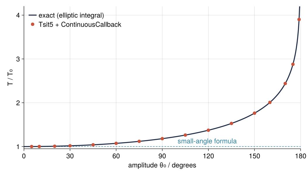
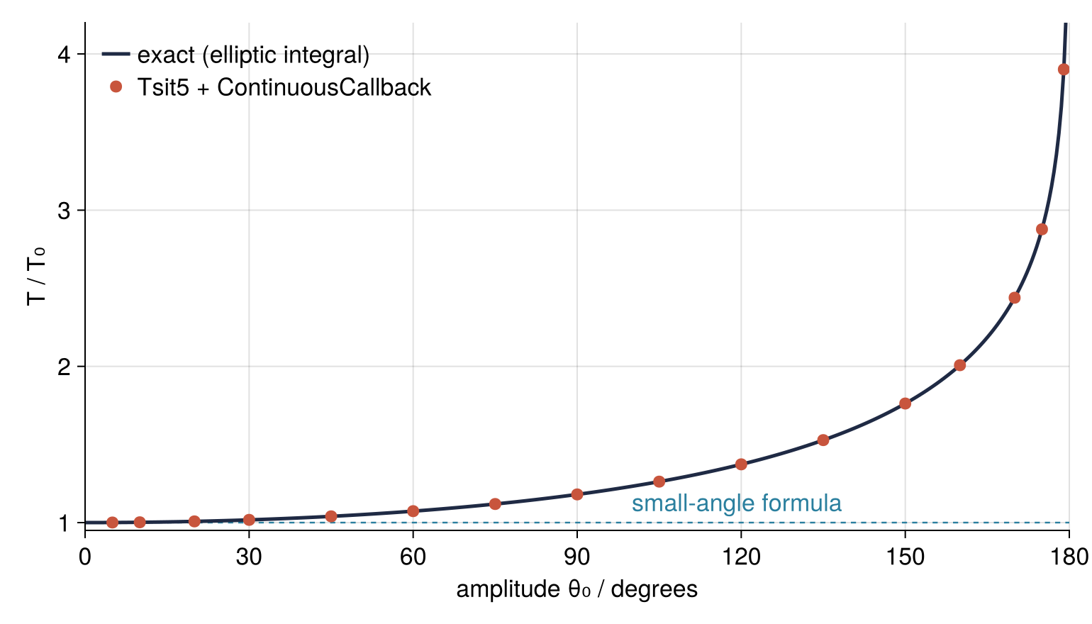
Period of a pendulum relative to the small-angle value, as a function of amplitude. Dots: DifferentialEquations.jl with a ContinuousCallback. Line: exact elliptic integral.

The period hardly moves for small amplitudes, is 18 % longer than the formula at 90°, and grows without bound as the amplitude nears 180°. Every dot is one call of solve with one callback that records zero crossings; the line is the elliptic integral. The six steps below build that figure.

Setup

DifferentialEquations.jl is the umbrella package of the SciML suite. Its ODE solvers live in OrdinaryDiffEq, which the umbrella loads and which is all this tutorial needs. With using DifferentialEquations instead, every line below runs unchanged. Install the packages once with import Pkg; Pkg.add(["OrdinaryDiffEq", "SpecialFunctions", "CairoMakie"]); Printf, which provides the formatted @printf, ships with Julia.

using OrdinaryDiffEq, SpecialFunctions, Printf, CairoMakie

const g, L = 9.81, 1.0     # m/s², m
T0 = 2π * sqrt(L / g)

const INK, ACCENT, SECOND, MUTED = "#1f2a44", "#c8553d", "#2a7f9e", "#8a8f98"
set_theme!(Theme(                          # the look of every figure below
    size = (770, 396), fontsize = 17,
    palette = (color = [INK, ACCENT, SECOND, MUTED],),
    Axis = (topspinevisible = false, rightspinevisible = false, xgridvisible = true, ygridvisible = true),
    Lines = (linewidth = 2.5,),
))

@printf("small-angle period T0 = %.4f s\n", T0)

small-angle period T0 = 2.0061 s

Step 1: Write the equation the way ODEProblem wants it

The solvers work on systems of first-order equations. The pendulum becomes one with the angular velocity \(\omega = \dot\theta\) as a second unknown:

\[\dot\theta = \omega, \qquad \dot\omega = -\frac{g}{L}\sin\theta .\]

The state is the vector \(u = (\theta, \omega)\). The right-hand side is a function of (du, u, p, t), time last, that fills the array du with the derivatives instead of returning a new array, which saves an allocation in every call. The ! in the name is the Julia convention for a function that changes one of its arguments. Parameters arrive in p, here a NamedTuple:

function pendulum!(du, u, p, t)
    (; g, L) = p
    θ, ω = u
    du[1] = ω
    du[2] = -(g / L) * sin(θ)
    return nothing
end

p = (g = g, L = L)

(g = 9.81, L = 1.0)

The line (; g, L) = p is destructuring: it creates local variables g and L from the fields of p with those names. The function never reads the globals of the setup, so it serves a pendulum of any length. The result travels in du, hence return nothing. Assigning to du instead of filling it is the first pitfall below.

Step 2: Build the problem, solve it, and look at what comes back

An ODEProblem bundles the function, the initial state, the time span as a tuple of floats, and the parameters. Tsit5() is a Runge-Kutta method by Tsitouras and the suite's recommended choice for problems that are not stiff, a term the pitfalls explain.

Tsit5 chooses its own step sizes. Each step computes the new state twice, with a fifth-order and a fourth-order formula from the same function calls (order \(p\): the error falls like the \(p\)-th power of the step size), and their difference estimates the error of that step. Below the tolerance, the step is accepted, and the same estimate sets the size of the next one, longer when the error came out small; above it, the step is rejected and retried shorter. Start the pendulum at rest at 90° and run it for 10 s:

θ0 = deg2rad(90)
prob = ODEProblem(pendulum!, [θ0, 0.0], (0.0, 10.0), p)
sol = solve(prob, Tsit5())

retcode: Success
Interpolation: specialized 4th order "free" interpolation
t: 40-element Vector{Float64}:
  0.0
  0.00010187194548975726
  0.0037377456926674644
  0.033393680304388704
  0.10877418485317376
  0.2261492158312155
  0.37052627720436604
  0.5554611081240757
  0.725826457812226
  0.9007319291660001
  1.1175669924029477
  1.3889698009400586
  1.6575355659427355
  ⋮
  6.836058632623079
  7.1137859716388405
  7.466677486684448
  7.814643139172066
  8.091376870554486
  8.51737565635596
  8.758093820622388
  9.102686196256958
  9.327083368482993
  9.703947150506485
  9.994777989476935
 10.0
u: 40-element Vector{Vector{Float64}}:
 [1.5707963267948966, 0.0]
 [1.57079627589133, -0.0009993637852545182]
 [1.5707278003011642, -0.03666728522784929]
 [1.5653265809455492, -0.32759102369300735]
 [1.5127677529425931, -1.0667154567230712]
 [1.3204622582488623, -2.2046354920195275]
 [0.9073446052289471, -3.476028723570032]
 [0.16130277507811205, -4.400594520495549]
 [-0.5760479198869191, -4.056326950128128]
 [-1.1794612309927808, -2.735536381945173]
 [-1.5491810709986704, -0.6507741793526645]
 [-1.3648143854227754, 2.003144582926861]
 [-0.5123603337560373, 4.13524976492996]
 ⋮
 [1.2288288835953645, 2.5009766381792713]
 [1.5523316054197414, -0.19186245094365614]
 [0.8854865980940838, -3.4782205890177993]
 [-0.5597362827259237, -4.041138281744828]
 [-1.3926066918100912, -1.780112514977942]
 [-1.2640703570920786, 2.3683892666393893]
 [-0.4539639794258338, 4.161448195697887]
 [0.9609199773988701, 3.3020577738210037]
 [1.4763372155926522, 1.2310906121611902]
 [1.2454722682711343, -2.436586522123279]
 [0.2082253532599297, -4.34298327564366]
 [0.1855195893193715, -4.3530036240346925]

retcode: Success says the solver reached the end. The two lists of 40 entries are t, the times at which accepted steps ended, and u, the states there. Count the work:

println(length(sol.t), " stored points, ", sol.stats.naccept, " accepted and ",
        sol.stats.nreject, " rejected steps, ", sol.stats.nf, " calls of pendulum!")
println(round.(sol.t[1:8], digits = 4))

40 stored points, 39 accepted and 4 rejected steps, 261 calls of pendulum!
[0.0, 0.0001, 0.0037, 0.0334, 0.1088, 0.2261, 0.3705, 0.5555]

The 40 points are the start plus one per accepted step. The first step, 0.0001 s, is a cautious guess; its error came out far below the tolerance, and the steps grew to about a quarter second. The four rejected steps are the controller asking for too much and backing off, which costs calls but leaves no trace. sol.u[k] is the state at sol.t[k], and sol[1, :] is θ at every stored time:

fig = Figure()
ax = Axis(fig[1, 1], xlabel = "t / s", ylabel = "θ / degrees", yticks = -90:45:90)   # row 1, column 1 of the figure's grid
lines!(ax, sol.t, rad2deg.(sol[1, :]), color = ACCENT)
scatter!(ax, sol.t, rad2deg.(sol[1, :]), color = ACCENT, markersize = 8)
fig

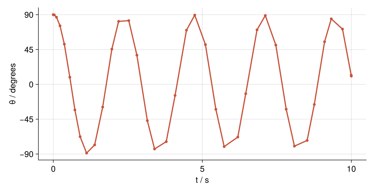
The curve is angular because only the ends of the steps are stored. The solver knows the motion in between just as well.

Step 3: Get the solution where you want it

A solution is callable. sol(t) evaluates it anywhere in the span through an interpolation that solve keeps by default and that is as accurate as the steps. It returns the whole state, and idxs = 1 restricts it to θ:

println(sol(0.5))
@printf("θ at 0.5, 1.0, 1.5 s: %.2f°, %.2f°, %.2f°\n", rad2deg.(sol([0.5, 1.0, 1.5]; idxs = 1))...)

[0.40176568395405404, -4.249418180043313]
θ at 0.5, 1.0, 1.5 s: 23.02°, -80.50°, -62.14°

At 0.5 s the bob is at 0.4018 rad, 23°, and moving toward the bottom at 4.25 rad/s. For a table or a plot on a fixed grid, saveat stores the solution at evenly spaced times instead:

sol_grid = solve(prob, Tsit5(); saveat = 0.02)
println(length(sol_grid.t), " stored points, ", sol_grid.stats.nf, " calls of pendulum!")
@printf("θ(0.51) = %.5f rad from the grid, %.5f rad from the full solution\n",
        sol_grid(0.51)[1], sol(0.51)[1])

501 stored points, 261 calls of pendulum!
θ(0.51) = 0.35891 rad from the grid, 0.35909 rad from the full solution

501 points for the same 261 calls: the steps did not change, only what is kept. The accurate interpolation needs the seven slopes Tsit5 computes inside each step, which saveat discards, so between grid points sol_grid falls back to a cruder one, already off in the third digit. Use saveat for a grid you know in advance and the plain solution for evaluation anywhere.

Step 4: Control the accuracy

The tolerance of Step 2 is reltol and abstol: a step is accepted when its error estimate stays below abstol + reltol * |u|. The defaults, reltol = 1e-3 and abstol = 1e-6, ask for three significant digits per step, and over a long run the errors of many steps add up.

The pendulum carries its own test, the energy per unit mass

\[E = \tfrac12 L^2\omega^2 + gL(1-\cos\theta),\]

which the true motion conserves. remake copies the problem with one field changed, here a span of 100 s, about forty swings. Three tolerance pairs with Tsit5, and the tightest once more with Vern9(), a ninth-order Runge-Kutta method by Verner:

energy(u) = 0.5 * L^2 * u[2]^2 + g * L * (1 - cos(u[1]))
prob100 = remake(prob; tspan = (0.0, 100.0))

for (alg, rtol, atol) in [(Tsit5(), 1e-3, 1e-6), (Tsit5(), 1e-6, 1e-9),
                          (Tsit5(), 1e-10, 1e-12), (Vern9(), 1e-10, 1e-12)]
    s = solve(prob100, alg; reltol = rtol, abstol = atol)
    E = energy.(s.u)
    drift = maximum(abs.(E .- E[1])) / E[1]
    @printf("%-5s reltol=%-6g abstol=%-6g nf=%6d  max energy drift %.1e\n",
            nameof(typeof(alg)), rtol, atol, s.stats.nf, drift)   # the bare name, without type parameters
end

Tsit5 reltol=0.001  abstol=1e-06  nf=  2049  max energy drift 1.6e-01
Tsit5 reltol=1e-06  abstol=1e-09  nf=  8529  max energy drift 9.9e-06
Tsit5 reltol=1e-10  abstol=1e-12  nf= 54153  max energy drift 2.4e-10
Vern9 reltol=1e-10  abstol=1e-12  nf= 18162  max energy drift 1.8e-10

The first line is the defaults, and the energy is off by 16 %. Whatever the solver traced there, it is not the pendulum of Step 1. Four times as many calls bring the drift to a thousandth of a percent, twenty-six times as many to 2.4e-10. At the tightest setting Vern9 gets there with a third of the calls: once the tolerance is tight, a higher order pays.

Do not trust the defaults with anything you plot, measure, or publish. Pass reltol = 1e-8, abstol = 1e-10 and loosen them only when the run time hurts. Near zero, reltol * |u| vanishes and abstol alone sets the bar, so pick it 100 to 1,000 times below the smallest value of that component you care about. With nothing conserved to watch, tighten both tolerances by a factor of ten and run again: if the result changes, the first run had not converged.

Step 5: Find the period with a ContinuousCallback

The period is the time between two passages through θ = 0 in the same direction. The solver can find them while it runs. It advances an object called the integrator, the running state of the solver, one step at a time: integrator.t is the current time, integrator.u the current state, integrator.p the parameters. A callback receives the integrator at the moment it fires, so integrator.t is then the time of the event; sol.t exists only after the run.

A ContinuousCallback takes three functions. The condition, here u[1], is the quantity whose zeros you want, and the solver locates each one by root finding on the interpolation inside a step. The second function, the affect, runs when the condition crosses zero upward, the third when it crosses downward, and nothing there ignores those crossings. This affect records the time:

crossings = Float64[]
upward = ContinuousCallback((u, t, integrator) -> u[1],             # zero when θ = 0
                            integrator -> push!(crossings, integrator.t),
                            nothing)                                 # skip downward crossings
solve(remake(prob; tspan = (0.0, 20.0)), Tsit5(); callback = upward, reltol = 1e-8, abstol = 1e-10)
println(round.(crossings, digits = 4))
println("periods: ", round.(diff(crossings), digits = 6))

[1.7759, 4.1437, 6.5116, 8.8794, 11.2472, 13.6151, 15.9829, 18.3508]
periods: [2.367842, 2.367842, 2.367842, 2.367842, 2.367842, 2.367842, 2.367842]

Eight upward crossings in 20 s, seven periods, each 2.367842 s to six decimals. With an affect in the third place too, the downward crossings would land in the same list and halve every interval. Passing terminate! as the affect stops the integration at the event instead.

The exact period is \(T = 4\sqrt{L/g}\,K(m)\) with \(m = \sin^2(\theta_0/2)\) and \(K\) the complete elliptic integral of the first kind, a special function computed to machine precision, as sin is. SpecialFunctions provides it as ellipk(m); a textbook that writes \(K(k)\) uses \(k = \sqrt m\):

T_num = (crossings[end] - crossings[1]) / (length(crossings) - 1)   # the mean of diff(crossings)
T_exact = 4 * sqrt(L / g) * ellipk(sin(θ0 / 2)^2)
@printf("numeric %.7f s   exact %.7f s   T/T0 = %.4f\n", T_num, T_exact, T_exact / T0)

numeric 2.3678419 s   exact 2.3678419 s   T/T0 = 1.1803

All seven printed digits agree. At 90° the pendulum needs 18 % longer than the small-angle formula promises.

Step 6: Sweep the amplitude

Turn Step 5 into a function of the amplitude that builds its own crossings vector on every call; a global one would collect the crossings of all amplitudes. Released from rest, the bob passes zero going down first, so the upward crossings come at 3/4, 7/4, and 11/4 of a period. At 179°, where the period is nearly \(4\,T_0\), that is near 3, 7, and 11 \(T_0\): a span of \(12\,T_0\) holds three crossings, two periods. period.(amplitudes) broadcasts it over the vector:

function period(θ0_deg)
    crossings = Float64[]
    upward = ContinuousCallback((u, t, integrator) -> u[1],
                                integrator -> push!(crossings, integrator.t), nothing)
    prob = ODEProblem(pendulum!, [deg2rad(θ0_deg), 0.0], (0.0, 12T0), p)
    solve(prob, Tsit5(); callback = upward, reltol = 1e-8, abstol = 1e-10)
    return (crossings[end] - crossings[1]) / (length(crossings) - 1)
end

amplitudes = [5, 10, 20, 30, 45, 60, 75, 90, 105, 120, 135, 150, 160, 170, 175, 179]
T_num = period.(amplitudes)
T_exact = 4 * sqrt(L / g) .* ellipk.(sin.(deg2rad.(amplitudes) ./ 2) .^ 2)

a_fine = range(0, 179.9, length = 400)
T_fine = 4 * sqrt(L / g) .* ellipk.(sin.(deg2rad.(a_fine) ./ 2) .^ 2)

fig = Figure(size = (770, 440))
ax = Axis(fig[1, 1], xlabel = "amplitude θ₀ / degrees", ylabel = "T / T₀",
          limits = (0, 180, 0.95, 4.2))
lines!(ax, [0, 180], [1, 1], color = SECOND, linewidth = 1.2, linestyle = :dash)
text!(ax, 100, 1.04, text = "small-angle formula", color = SECOND, align = (:left, :bottom))
lines!(ax, a_fine, T_fine ./ T0, color = INK, label = "exact (elliptic integral)")
scatter!(ax, amplitudes, T_num ./ T0, color = ACCENT, markersize = 12, label = "Tsit5 + ContinuousCallback")
axislegend(ax, position = :lt, framevisible = false)
display(fig)                                     # a bare fig shows only as the last line of a cell

for (a, T) in zip(amplitudes[1:3:end], T_num[1:3:end])
    @printf("%4d°   T/T0 = %.4f\n", a, T / T0)
end
@printf("largest relative error %.1e\n", maximum(abs.(T_num ./ T_exact .- 1)))

   5°   T/T0 = 1.0005
  30°   T/T0 = 1.0174
  75°   T/T0 = 1.1190
 120°   T/T0 = 1.3729
 160°   T/T0 = 2.0075
 179°   T/T0 = 3.9011
largest relative error 1.7e-06

At 30° the small-angle formula is short by less than 2 %, close enough to earn its place in every textbook. At 75° the true period is 12 % longer, at 120° 37 %, at 160° twice as long. No dot misses the exact curve by more than 1.7e-6, far below the size of a marker.

Pitfalls

Rebinding du instead of filling it. Write the derivatives as a new array assigned to du, and the pendulum stays where it was released:

function pendulum_wrong!(du, u, p, t)
    θ, ω = u
    du = [ω, -(p.g / p.L) * sin(θ)]       # a new local array; the solver never sees it
    return nothing
end

s = solve(ODEProblem(pendulum_wrong!, [θ0, 0.0], (0.0, 10.0), p), Tsit5())
println(s.retcode, ", final state ", s.u[end])

Success, final state [1.5707963267948966, 0.0]

Success, no warning, and the final state is the initial one, 90° and at rest. The assignment makes the name du point to a new array inside the function, while the array the solver passed in is never written, so the slopes it reads stay at zero. Fill the array element by element, as in Step 1, or in one line with du .= ….

Reading sol[1] as the first state. sol[1] is one number, θ at the first time, not the state vector:

println(sol[1], "   ", sol.u[1], "   ", sol[:, 1])

1.5707963267948966   [1.5707963267948966, 0.0]   [1.5707963267948966, 0.0]

The solution indexes like a matrix with the components as rows and the stored times as columns, and a single index counts through its entries one by one, so sol[2] is ω at the first time. The state at the first time is sol.u[1] or sol[:, 1], and θ over all times is sol[1, :].

An explicit method on a stiff problem. A problem is stiff when it mixes time scales that lie far apart. The Van der Pol oscillator with μ = 200 is the classic case: it creeps along for long stretches and then snaps over within a fraction of a second. An explicit method such as Tsit5, which computes the next state from the current one alone, turns unstable with steps longer than the fastest time scale, so it keeps its steps short even where the solution hardly changes. The symptom is a step count far beyond what the shape of the solution suggests, growing in proportion to the time span, with maximum(diff(sol.t)) tiny:

function vdp!(du, u, p, t)
    μ = p[1]     # a plain vector, for which Rodas5P is precompiled; a NamedTuple works but compiles about 10 s on first use
    x, v = u
    du[1] = v
    du[2] = μ * (1 - x^2) * v - x
    return nothing
end

vdp = ODEProblem(vdp!, [2.0, 0.0], (0.0, 500.0), [200.0])
for alg in [Tsit5(), Rodas5P()]
    s = solve(vdp, alg; reltol = 1e-6, abstol = 1e-9)
    @printf("%-7s steps = %6d  calls = %7d  longest step = %.3f s\n",
            nameof(typeof(alg)), s.stats.naccept, s.stats.nf, maximum(diff(s.t)))
end

Tsit5   steps =  52413  calls =  314709  longest step = 0.043 s
Rodas5P steps =    822  calls =   10780  longest step = 5.763 s

Tsit5 takes about 52,000 steps and over 300,000 calls, none longer than 0.043 s. Rodas5P needs 822 steps, the longest 5.8 s. It is an implicit method: it solves an equation for the next state in every step and stays stable with long steps. The suite computes the Jacobian this requires by automatic differentiation, without being asked. When your counts look like the first line, switch to Rodas5P().

Variations

Damped and driven. Add γ, A, and Ω to p and \(-\gamma\omega + A\cos(\Omega t)\) to du[2]. With \(g/L = 1\), γ = 0.5, A near 1.2, and Ω = 2/3 the motion is chaotic, and its Poincaré section, the state recorded once every drive period, is saveat = t1:2π/Ω:t2, with t1 after the transient.
Projectile with air drag. Four components \((x, h, v_x, v_h)\), \(h\) being the height, and a drag force proportional to \(v^2\). The callback ContinuousCallback((u, t, integrator) -> u[2], nothing, terminate!) ends the run when the height crosses zero on the way down, and sol.u[end] is the landing state.
The double pendulum. Two angles, two angular velocities, and a right-hand side that fills half a page; nothing else changes. The energy check is no longer optional, because a sign error in that page is easy to make and hard to see.
An epidemic. The SIR model counts susceptible, infected, and recovered people in three components, with p = (β = …, γ = …). A condition that returns \(\dot I = \beta S I - \gamma I\), with β and γ read from integrator.p, fires the callback at the peak of the epidemic.

Cheat sheet

function f!(du, u, p, t)                         # fill du, never rebind it
    du[1] = …; du[2] = …; return nothing
end
prob = ODEProblem(f!, u0, (t0, t1), p)           # p: a NamedTuple of parameters
sol = solve(prob, Tsit5(); reltol = 1e-8, abstol = 1e-10)   # defaults 1e-3 / 1e-6 are too loose
#   Vern9() for tight tolerances, Rodas5P() for stiff problems; saveat = Δt for a fixed grid
sol(t), sol(t; idxs = i)                         # anywhere in the span; one component
sol.t, sol.u[k], sol[i, :]                       # stored times, state k, component i over time
cb = ContinuousCallback(cond, affect!, affect_neg!)   # cond(u, t, integrator) = 0; terminate! stops
sol.retcode, sol.stats.nf                        # Success?; cost meter