Fit a curve with error bars and draw a confidence band in Julia

The problem

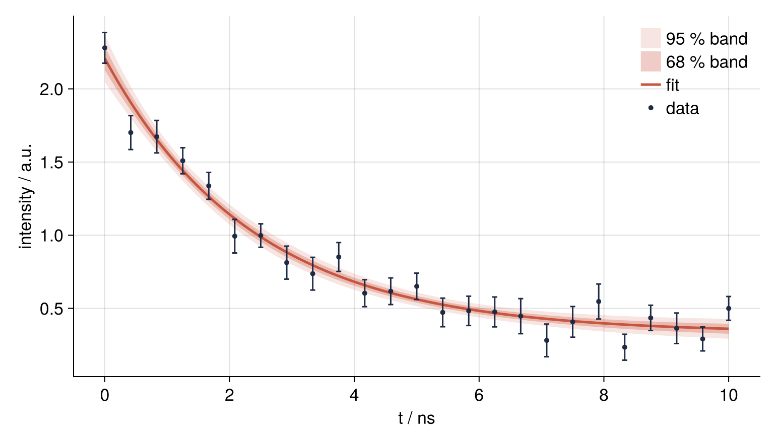
You have 25 readings \(y_i\) at times \(t_i\), every one with its own standard deviation \(\sigma_i\), and a model with a handful of free parameters. You want the parameters with errors you can stand behind, a plot of the data with error bars, and a confidence band that shows how tightly the data pin the fitted curve down. In Julia the fit is one call to curve_fit from LsqFit, and the band takes eight more lines.

The example is a fluorescence decay after a laser pulse, \(I(t) = A e^{-t/\tau} + B\), with \(\tau\) the lifetime and \(B\) the background. Swap in your own data and model and leave the rest of the cell alone.

The code

Copy

using LsqFit, LinearAlgebra, Printf, CairoMakie

# ---- data: replace these lines with your own t, y, sigma
# (drawn from A = 2.0, tau = 2.5, B = 0.3 plus Gaussian noise of width sigma)
t = collect(range(0, 10, length = 25))                       # ns
y = [2.2804, 1.7013, 1.6733, 1.5087, 1.3373, 0.9933, 0.9974, 0.8124, 0.7367, 0.8510, 0.6034, 0.6168, 0.6504,
     0.4720, 0.4828, 0.4755, 0.4466, 0.2808, 0.4076, 0.5467, 0.2343, 0.4347, 0.3636, 0.2908, 0.4995]
sigma = [0.1050, 0.1159, 0.1110, 0.0890, 0.0920, 0.1149, 0.0802, 0.1128, 0.1119, 0.0987, 0.0921, 0.0911, 0.0902,
         0.0978, 0.1002, 0.1021, 0.1198, 0.1117, 0.1049, 0.1196, 0.0886, 0.0864, 0.1045, 0.0818, 0.0814]

# ---- model and fit: replace model, names, and p0 with your own (one p0 entry per parameter)
# the model gets the whole vector t and the parameter vector p and must return a vector;
# @. makes every operation elementwise, so p[1] * t^2 + p[2] needs it too
model(t, p) = @. p[1] * exp(-t / p[2]) + p[3]
names = ["A", "tau", "B"]
p0 = [y[1] - y[end], 0.3 * t[end], y[end]]                   # rough guesses, taken from the data
w = PrecisionWeights(1 ./ sigma .^ 2)                        # the sigma are true standard deviations
fit = curve_fit(model, t, y, w, p0)
p = coef(fit)
C = vcov(fit)            # parameter covariance matrix; its diagonal holds the squared errors
perr = stderror(fit)
chi2_dof = sum(abs2, (y .- model(t, p)) ./ sigma) / (length(t) - length(p))

# ---- confidence band: propagate the parameter covariance through the model
tt = range(extrema(t)..., length = 300)                      # from the first t to the last
J = zeros(length(tt), length(p))   # d model / d parameter: how the curve moves when each parameter moves
for k in eachindex(p)
    dp = zeros(length(p))
    dp[k] = 1e-6 * max(abs(p[k]), 1.0)
    J[:, k] = (model(tt, p .+ dp) .- model(tt, p .- dp)) ./ (2 * dp[k])
end
band = [sqrt(dot(j, C, j)) for j in eachrow(J)]   # jᵀ C j for each row j of J: 1-sigma uncertainty of the curve

# ---- report and plot
for (name, val, err) in zip(names, p, perr)
    @printf("%-3s = %6.3f ± %.3f\n", name, val, err)
end
@printf("chi2 / dof = %.2f\n", chi2_dof)

curve = model(tt, p)
fig = Figure(size = (770, 440), fontsize = 17)
ax = Axis(fig[1, 1]; xlabel = "t / ns", ylabel = "intensity / a.u.", xticks = 0:2:10,
          topspinevisible = false, rightspinevisible = false)
band!(ax, tt, curve .- 2 .* band, curve .+ 2 .* band; color = ("#c8553d", 0.15), label = "95 % band")
band!(ax, tt, curve .- band, curve .+ band; color = ("#c8553d", 0.30), label = "68 % band")
lines!(ax, tt, curve; color = "#c8553d", linewidth = 2.5, label = "fit")
errorbars!(ax, t, y, sigma; color = "#1f2a44", linewidth = 1.5, whiskerwidth = 5)
scatter!(ax, t, y; color = "#1f2a44", markersize = 7, label = "data")
axislegend(ax; framevisible = false)
fig

A   =  1.876 ± 0.077
tau =  2.380 ± 0.229
B   =  0.332 ± 0.043
chi2 / dof = 0.93

The knobs

The weights decide what the errors mean. PrecisionWeights(1 ./ sigma .^ 2) declares each \(\sigma_i\) to be the true standard deviation of its reading, and curve_fit minimizes \(\sum_i \left((y_i - f(t_i))/\sigma_i\right)^2\). The docstring calls this case "scale known": vcov comes from the weights alone, so the errors are absolute. AnalyticWeights with the same numbers treats them as relative and multiplies every error by \(\sqrt{\chi^2/\text{dof}}\), which forces the reduced chi-square to one. On this data that gives 0.075, 0.221 and 0.041 instead of 0.077, 0.229 and 0.043, close because χ²/dof is already 0.93. Use precision weights whenever you trust your \(\sigma_i\) as standard deviations, and analytic weights only when you trust their ratios. From Python, this is SciPy's absolute_sigma=True, as in the SciPy version of this recipe.

The starting values come from the data: \(A\) at the fall from first to last reading, \(B\) at the last reading, \(\tau\) at 30 % of the time span. The data were drawn from \(A = 2.0\), \(\tau = 2.5\) and \(B = 0.3\), and the fit misses them by 1.6, 0.5 and 0.8 standard errors. That is about how far honest one-sigma errors should miss.

The band answers a different question: where is the curve itself? \(C\), from vcov, is the parameter covariance: its diagonal holds the squared errors, and its off-diagonal entries say how errors in \(A\), \(\tau\) and \(B\) move together. For each \(t\) on the curve, a vector \(j\) holds the derivatives of the model with respect to each parameter, and these vectors are the rows of \(J\). First-order error propagation gives the variance of the curve at that \(t\) as

which is the one-variable rule \((\partial f/\partial p)^2 \sigma_p^2\) with the correlations included. The cell builds \(J\) by central differences, so you never differentiate your model by hand. The variable band holds \(\sigma_\text{curve}\): once it is the 68 % band, twice the 95 % band, and across this data it runs from 0.023 to 0.080. It says nothing about the next reading. For that, add the standard deviation \(\sigma(t)\) you expect of a single reading at \(t\), here 0.08 to 0.12: the prediction band \(\sqrt{\sigma_\text{curve}^2(t) + \sigma^2(t)}\) does not narrow as you add points.

Pitfalls

Starting values in the wrong units. Put the time axis in picoseconds, so that it runs to 10 000, and start \(\tau\) at 1. Then \(e^{-t/\tau}\) is below \(10^{-180}\) at every point after the first, and no change in \(\tau\) is visible to the fit. LsqFit does not complain. On this data fit.converged is true, \(\tau\) comes back as exactly 1.0, and stderror gives Inf for it, with nothing printed. The check is therefore yours: look for Inf or NaN in stderror(fit) and compare coef(fit) with p0, because a parameter that has not moved was never fitted. Take p0 from the data, as the cell does.

A reduced chi-square far from one. With honest error bars and the right model, χ²/dof sits near one; here it is 0.93. At 15 the points scatter about four times farther from the curve than your \(\sigma_i\) claim (\(\sqrt{15} \approx 3.9\)): either the \(\sigma_i\) are underestimated or the model misses something, and the errors from precision weights are too small until you know which. Switching to AnalyticWeights makes the number go away but not the problem, which now hides in a rescaling. At 0.1 the scatter is a third of your \(\sigma_i\), so they are about three times too large, and every error you report is inflated by the same factor.

Reading the band as a prediction. Only nine of the 25 points lie inside the 68 % band, and that is correct: 25 readings together pin the mean curve down far better than any one of them. Add each point's own \(\sigma_i\) in quadrature and 18 of the 25 fall inside, against the 17 that 68 % predicts.