Eigenvalues with numpy.linalg: normal modes of coupled oscillators

Afterwards you can turn a physical system into a matrix, solve it with numpy.linalg.solve, pick eigh or eig, and check eigenvectors by what they must satisfy.

Topic: Linear algebra
Field: Chemistry, Engineering, Physics
Libraries: matplotlib 3.11.2, numpy 2.5.3
Prerequisites: none beyond Python basics
Notebook: Download py-eigenvalues-numpy.ipynb, executed with the versions above

The problem: the normal modes of three coupled gliders

Three gliders of 200 g sit 0.5 m apart on an air track, joined to each other and to two end posts by four springs of 10 N/m. Pull the first one with 1 N, hold it until everything is still, and let go. The motion that follows is a mess, and it never repeats. Hidden in it are three patterns in which all gliders move at the same frequency, the normal modes, and finding them is an eigenvalue problem that numpy.linalg solves in one call.

Newton's second law for the three displacements fits in one line,

\[m\,\ddot{\mathbf x} = -K\,\mathbf x ,\]

with \(m\) the mass of a glider and \(K\) a 3 × 3 matrix built from the springs. The normal modes of the gliders come out at 0.86, 1.59, and 2.08 Hz.

Take the posts away and put atoms in place of the gliders, and the same construction describes a carbon dioxide molecule along its axis. With its bond spring fitted to the center of one infrared band, the model predicts the center of the same band for carbon-13 dioxide at 2282.2 cm⁻¹, in wavenumbers, the spectroscopists' unit. Measured, it is 2283.5 cm⁻¹. An engineer uses the same construction for the floors of a three-story building.

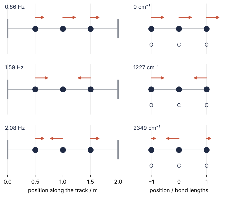
Normal modes of three gliders between two posts (left) and of a CO₂ molecule (right), slowest at the top. Arrows: how far each mass moves in that mode. Frequencies printed in each panel: 0.86, 1.59, 2.08 Hz and 0, 1227, 2349 cm⁻¹.

Both systems end up in this picture, the three modes of each with an arrow for how far every mass moves. Every arrow and every frequency in it comes from np.linalg.eigh, and the six steps below build it from the springs up.

Setup

One glider on one spring would oscillate at 7.071 rad/s, which the setup prints as a check.

import numpy as np
import matplotlib.pyplot as plt

m = 0.200   # kg, one glider
k = 10.0    # N/m, one spring

plt.rcParams.update({                      # the look of every figure below
    "figure.figsize": (7, 3.6), "figure.dpi": 110,
    "axes.spines.top": False, "axes.spines.right": False,
    "axes.grid": True, "grid.alpha": 0.25,
    "font.size": 11, "lines.linewidth": 1.8,
})
INK, ACCENT, SECOND, MUTED = "#1f2a44", "#c8553d", "#2a7f9e", "#8a8f98"

print(f"one glider on one spring: sqrt(k/m) = {np.sqrt(k / m):.3f} rad/s")

one glider on one spring: sqrt(k/m) = 7.071 rad/s

Step 1: Write Newton's equations as one matrix equation

Glider 1 feels the left spring \(k_1\), stretched by \(x_1\), and the spring \(k_2\) to glider 2, stretched by \(x_2 - x_1\):

\[m\,\ddot x_1 = -k_1 x_1 + k_2\,(x_2 - x_1) = -(k_1 + k_2)\,x_1 + k_2\,x_2 .\]

One such row per glider gives \(m\ddot{\mathbf x} = -K\mathbf x\). stiffness builds \(K\) from the spring constants, left post to right post, 0 for a free end, and np.diag(v, 1) puts v just above the diagonal. It is a function because Step 5 reuses it.

def stiffness(springs):
    """Stiffness matrix of masses in a line; springs from left to right, 0 for a free end."""
    s = np.asarray(springs, dtype=float)
    return np.diag(s[:-1] + s[1:]) - np.diag(s[1:-1], 1) - np.diag(s[1:-1], -1)

K = stiffness([k, k, k, k])     # post, glider 1, glider 2, glider 3, post
print(K, "N/m")

[[ 20. -10.   0.]
 [-10.  20. -10.]
 [  0. -10.  20.]] N/m

The diagonal holds the sum of the two springs on each glider, 20 N/m, and the entries beside it minus the spring between neighbors, −10 N/m. \(K\) is symmetric because a spring pulls both its ends equally hard.

Step 2: Find the starting position with solve

Held with 1 N, the gliders sit where the springs balance the pull, \(K\mathbf x_0 = \mathbf F\). That is a linear system, the job of np.linalg.solve:

F = np.array([1.0, 0.0, 0.0])          # N, the pull on glider 1
x0 = np.linalg.solve(K, F)

print("x0 =", np.round(100 * x0, 2), "cm")
print("K @ x0 equals F:", np.allclose(K @ x0, F))
print(f"left spring {k * x0[0]:.2f} N, right spring {k * x0[2]:.2f} N")

x0 = [7.5 5.  2.5] cm
K @ x0 equals F: True
left spring 0.75 N, right spring 0.25 N

Glider 1 moves 7.5 cm, the others 5.0 and 2.5 cm, and the two end springs share the 1 N as 0.75 N and 0.25 N. Use solve, not np.linalg.inv(K) @ F. The inverse is the solution of \(KX = 1\), one solve for every column of the identity, and the product with \(\mathbf F\) comes on top, so you pay for three right-hand sides to use one.

Step 3: Ask eigh for the normal modes

Try a motion in which every glider oscillates at one frequency, with its own amplitude: \(\mathbf x(t) = \mathbf a\cos\omega t\). Then \(\ddot{\mathbf x} = -\omega^2\mathbf x\), and Newton's law becomes

\[\frac{K}{m}\,\mathbf a = \omega^2\,\mathbf a .\]

\(K/m\) leaves the direction of \(\mathbf a\) alone and only stretches it, by \(\omega^2\). A vector that a matrix only stretches is called an eigenvector, and the stretch factor its eigenvalue. Here the eigenvalue is the squared frequency of a mode and the eigenvector its pattern.

np.linalg.eigh handles symmetric matrices (Hermitian, in its documentation). It returns the eigenvalues in ascending order and a matrix whose columns are the eigenvectors, perpendicular to each other and of unit length:

w2, V = np.linalg.eigh(K / m)           # eigenvalues are omega squared
omega = np.sqrt(w2)                     # rad/s
f = omega / (2 * np.pi)                 # Hz
f_exact = np.sqrt(k / m * np.array([2 - np.sqrt(2), 2, 2 + np.sqrt(2)])) / (2 * np.pi)

print("w2   :", np.round(w2, 2), "1/s^2")
print("eigh :", np.round(f, 3), "Hz")
print("exact:", np.round(f_exact, 3), "Hz")
with np.printoptions(precision=3, suppress=True):
    print(V)

w2   : [ 29.29 100.   170.71] 1/s^2
eigh : [0.861 1.592 2.079] Hz
exact: [0.861 1.592 2.079] Hz
[[-0.5   -0.707  0.5  ]
 [-0.707  0.    -0.707]
 [-0.5    0.707  0.5  ]]

The frequencies, 0.861, 1.592, and 2.079 Hz, agree with the closed form \(\omega^2 = (k/m)\,(2 - \sqrt2,\ 2,\ 2 + \sqrt2)\) to every printed digit. Read V by columns. In the first, all gliders move together, the middle one √2 times as far. In the second, the middle one stands still and the outer two move against each other. In the third, the middle one moves against the outer two. In this run the first column came back all negative, the same mode, as the first pitfall explains.

Step 4: Check the eigenvectors and rebuild the motion

Each column must obey \((K/m)\,\mathbf v = \omega^2\mathbf v\), so together \((K/m)\,V = V\,\mathrm{diag}(\omega^2)\), and as perpendicular unit vectors \(V^\mathsf{T}V = 1\), the identity matrix. Check both first:

residual = np.abs(K / m @ V - V @ np.diag(w2)).max()
print(f"largest entry of (K/m) V - V diag(w2): {residual:.0e} 1/s^2")
print(f"largest entry of V^T V - 1:           {np.abs(V.T @ V - np.eye(3)).max():.0e}")

largest entry of (K/m) V - V diag(w2): 3e-14 1/s^2
largest entry of V^T V - 1:           8e-16

The residual is of order 10⁻¹⁴ s⁻² against eigenvalues up to 171 s⁻², and \(V^\mathsf{T}V\) misses the identity by 10⁻¹⁵. Both are rounding.

The equation is linear, so every motion is the three modes added up, each with its own amplitude \(c_n\), and a start from rest needs only the cosines:

\[\mathbf x(t) = \sum_n c_n\,\mathbf v_n \cos\omega_n t .\]

The patterns are perpendicular unit vectors, so \(c_n = \mathbf v_n\cdot\mathbf x_0\), and V.T @ x0 gives all three. In the code, [:, None] turns c and omega into columns, so row \(n\) of the product holds c[n] * cos(omega[n] * t) at each of the 1001 times, and V @ turns that 3 × 1001 array into displacements. A second release starts from (5, 0, −5) cm, the second pattern itself, to show one mode alone.

c = V.T @ x0                            # amplitude of each mode in the start
print("c =", np.round(100 * c, 2), "cm")
print(f"frequency ratios: {f[1] / f[0]:.3f} and {f[2] / f[0]:.3f}")

t = np.linspace(0, 10, 1001)            # s
x = V @ (c[:, None] * np.cos(omega[:, None] * t))
x0_pure = np.array([0.05, 0.0, -0.05])  # m
x_pure = V @ ((V.T @ x0_pure)[:, None] * np.cos(omega[:, None] * t))

fig, axes = plt.subplots(2, 1, figsize=(7, 4.4), sharex=True)
for ax, xs, color in [(axes[0], x, INK), (axes[1], x_pure, ACCENT)]:
    for n, offset in enumerate([20, 0, -20]):
        ax.axhline(offset, color=MUTED, lw=1)
        ax.plot(t, 100 * xs[n] + offset, color=color)
        ax.text(10.15, offset, f"glider {n + 1}", va="center", color=color)
    ax.set(ylabel="displacement / cm", ylim=(-30, 35), yticks=[-20, 0, 20])
axes[1].text(0.15, 28, f"{f[1]:.2f} Hz", va="bottom", color=ACCENT)
axes[1].set(xlabel="t / s", xlim=(0, 10))
plt.show()

c = [-8.54 -3.54  1.46] cm
frequency ratios: 1.848 and 2.414

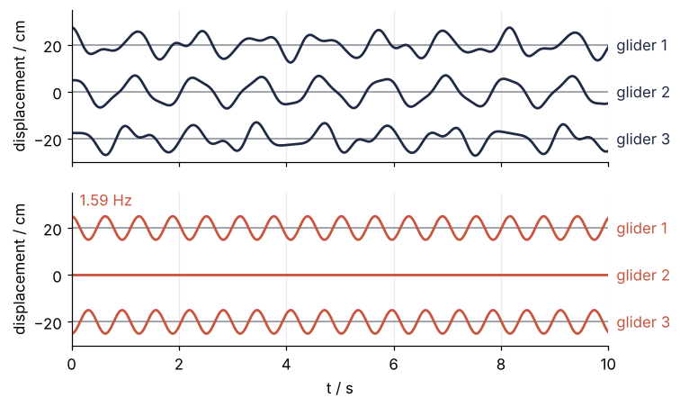
The slow mode carries most of the start, 8.54 cm against 3.54 and 1.46 cm, whatever signs eigh chose. The plot shifts the gliders by 20 cm, with gray lines at their rest positions. The upper panel never repeats, because the frequency ratios, 1.848 and 1 + √2 = 2.414, are irrational. In the lower one each glider runs one cosine at 1.59 Hz, and glider 2 never moves. That is a normal mode.

Step 5: Choose between eig and eigh when the masses differ

Without posts the same function describes O=C=O, its bonds the springs. For now the springs are 1 and the masses in u, the atomic mass unit, so the eigenvalues are plain numbers. With unequal masses Newton's law reads \(M\ddot{\mathbf x} = -K\mathbf x\), with \(M\) the diagonal matrix of the masses. Dividing row \(i\) by \(m_i\), Step 4's column trick in K1 / m_co2[:, None], gives \(A = M^{-1}K\), which is not symmetric. Here the two functions part ways:

m_co2 = np.array([15.994915, 12.0, 15.994915])   # u: 16O, 12C, 16O (NIST atomic masses)
K1 = stiffness([0, 1, 1, 0])                     # no posts, springs of 1
A = K1 / m_co2[:, None]                          # row i divided by m_i

w, V_eig = np.linalg.eig(A)
with np.printoptions(precision=4, suppress=True):
    print("eig :", w, w.dtype)
    print("eigh:", np.linalg.eigh(A)[0])
print(f"dot product of eig's first and last vector: {(V_eig[:, 0] @ V_eig[:, 2]).real:.3f}")

eig : [ 0.2292+0.j  0.0625+0.j -0.    +0.j] complex128
eigh: [-0.0019  0.0625  0.2311]
dot product of eig's first and last vector: -0.127

eig gets the values right, 0.2292, 0.0625, and 0, in no promised order and as complex numbers, since a matrix that is not symmetric can have complex eigenvalues. Its vectors are not perpendicular either (a dot product of −0.127), so Step 4's amplitudes would come out wrong. eigh raises no warning and gets the outer two wrong, −0.0019 and 0.2311, because it reads only the lower triangle and mirrors it.

The fix is a symmetric matrix with the same frequencies. Write Newton's law in components and substitute \(q_i = \sqrt{m_i}\,x_i\):

\[m_i\,\ddot x_i = -\sum_j K_{ij}\,x_j \quad\Longrightarrow\quad \ddot q_i = -\sum_j \frac{K_{ij}}{\sqrt{m_i m_j}}\,q_j .\]

The matrix in the sum, \(D\), is symmetric because \(K\) is, and it describes the same motion, so it has the same \(\omega^2\). np.outer(m_co2, m_co2) holds the products \(m_i m_j\), so \(D\) is one line:

D = K1 / np.sqrt(np.outer(m_co2, m_co2))         # K_ij / sqrt(m_i m_j)
w2_co2, Q = np.linalg.eigh(D)
X = Q / np.sqrt(m_co2)[:, None]                  # back from q to displacements x

with np.printoptions(precision=4, suppress=True):
    print("eigh(D):", w2_co2)
print(f"1/m_O = {1 / m_co2[0]:.4f},  1/m_O + 2/m_C = {1 / m_co2[0] + 2 / m_co2[1]:.4f}")

eigh(D): [0.     0.0625 0.2292]
1/m_O = 0.0625,  1/m_O + 2/m_C = 0.2292

Now eigh returns 0, 0.0625, and 0.2292, in order. The middle value is \(1/m_\mathrm{O}\), an oxygen on one spring around a resting carbon, and the last is \(1/m_\mathrm{O} + 2/m_\mathrm{C}\). The columns of X are the displacement patterns. If the matrix can be made symmetric, do it and use eigh. eig is for matrices that cannot be, such as those of damped systems.

Step 6: Read the eigenvalues as a CO₂ spectrum

Infrared spectra are quoted in wavenumbers, \(\tilde\nu = f/c\) with \(c\) the speed of light, in cm⁻¹. A real spring \(k\) turns Step 5's plain-number eigenvalues \(\lambda\) into \(\omega^2 = \lambda\,k/u\), with \(u = 1.66054 \times 10^{-27}\) kg and \(k/u\) in s⁻², so the units close. The fastest mode, the carbon against both oxygens, is the asymmetric stretch, with the largest eigenvalue, \(\lambda_3\) = w2_co2[2]. In ¹²C¹⁶O₂ its band origin, the band's center, is at \(\tilde\nu_3 = 2349.1\) cm⁻¹ (HITRAN), so \(k = (2\pi c\,\tilde\nu_3)^2\,u/\lambda_3\).

wavenumbers repeats Step 5 in SI units and clips at zero: the zero mode can come out a hair below zero, like eig's −0., and np.sqrt would return nan.

u = 1.66054e-27          # kg, atomic mass constant (CODATA)
c_cm = 2.99792458e10     # cm/s, speed of light, exact in SI
nu3_12 = 2349.1          # cm^-1, band origin of the asymmetric stretch of 12C16O2 (HITRAN lines)
k_bond = (2 * np.pi * c_cm * nu3_12) ** 2 * u / w2_co2[2]
print(f"k = {k_bond:.0f} N/m")

def wavenumbers(masses_u, k_bond):
    """Normal-mode wavenumbers in cm^-1 of three atoms in a line, joined by two springs."""
    mass = np.asarray(masses_u) * u
    D = stiffness([0, k_bond, k_bond, 0]) / np.sqrt(np.outer(mass, mass))
    w2 = np.linalg.eigh(D)[0]
    return np.sqrt(np.clip(w2, 0, None)) / (2 * np.pi * c_cm)

m_13 = np.array([15.994915, 13.003355, 15.994915])   # u: 16O, 13C, 16O (NIST atomic masses)
nu3_13_measured = 2283.5                              # cm^-1, band origin of the same band in 13C16O2 (HITRAN lines)
print("12C16O2:", ", ".join(f"{nu:.1f}" for nu in wavenumbers(m_co2, k_bond)), "cm^-1")
print(f"13C16O2: model {wavenumbers(m_13, k_bond)[2]:.1f} cm^-1, measured {nu3_13_measured:.1f} cm^-1")

k = 1419 N/m
12C16O2: 0.0, 1226.9, 2349.1 cm^-1
13C16O2: model 2282.2 cm^-1, measured 2283.5 cm^-1

The spring is 1419 N/m. The modes are 0 for the molecule sliding as a whole, 1226.9 cm⁻¹ for the oxygens moving against each other with the carbon still, and 2349.1 cm⁻¹ for the asymmetric stretch. The middle one is the model's, not a measurement, and the last confirms nothing: the spring was fitted to it.

The test is carbon-13. Its bonds are the same electrons, so the spring stays, and the model predicts 2282.2 cm⁻¹ against a measured 2283.5 cm⁻¹. The spring cancels in the ratio of the two origins, since \(\lambda\) depends on the masses alone: the agreement tests Step 5's mass weighting, not the fit. The remaining 1.3 cm⁻¹ is the bond not being a perfect harmonic spring.

The next cell draws the picture at the top. Since an eigenvector is fixed only up to a factor, sign_fixed picks one: largest component 1, first component positive.

def sign_fixed(v):
    """Scale a mode to a largest component of 1, with the first component positive."""
    v = v / np.abs(v).max()
    return v if v[0] > 0 else -v

def draw_mode(ax, rest, mode, scale, label, names=(), posts=()):
    ends = posts if posts else (rest[0], rest[-1])
    ax.plot(ends, [0, 0], color=MUTED, lw=1)                       # the springs
    for p in posts:
        ax.plot([p, p], [-0.35, 0.35], color=MUTED, lw=3)
    ax.plot(rest, np.zeros(3), "o", color=INK, ms=11, zorder=3)
    for r, d in zip(rest, sign_fixed(mode)):
        if abs(d) > 1e-6:                                          # a mass at rest gets no arrow
            ax.annotate("", xy=(r + scale * d, 0.45), xytext=(r, 0.45),
                        arrowprops=dict(arrowstyle="-|>", color=ACCENT, lw=1.8,
                                        shrinkA=0, shrinkB=0))
    for r, name in zip(rest, names):
        ax.text(r, -0.5, name, ha="center", va="top", color=INK)
    ax.text(0.0, 1.0, label, transform=ax.transAxes, va="top", color=INK)
    ax.set(ylim=(-1, 1), yticks=[])
    ax.spines["left"].set_visible(False)

nu = wavenumbers(m_co2, k_bond)
fig, axes = plt.subplots(3, 2, figsize=(8, 6.3), sharex="col", width_ratios=(4.2, 3.3))
fig.subplots_adjust(wspace=0.12)        # widths follow the x ranges: masses equally spaced
for n in range(3):
    draw_mode(axes[n, 0], [0.5, 1.0, 1.5], V[:, n], 0.24, f"{f[n]:.2f} Hz", posts=(0.0, 2.0))
    draw_mode(axes[n, 1], [-1, 0, 1], X[:, n], 0.48, f"{nu[n]:.0f} cm⁻¹", names=("O", "C", "O"))
for ax in axes[:2].flat:                                           # one x axis per column
    ax.spines["bottom"].set_visible(False)
    ax.tick_params(bottom=False)
axes[2, 0].set(xlabel="position along the track / m", xlim=(-0.05, 2.05))
axes[2, 1].set(xlabel="position / bond lengths", xlim=(-1.65, 1.65))
plt.show()

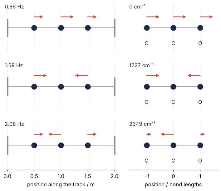
Row by row the arrows of both columns point the same ways, in different lengths, and the light carbon moves far in the bottom row so the center of mass stays put.

Pitfalls

Comparing eigenvectors by their sign. In Step 3 the in-phase mode, all gliders together, came back as (−0.5, −0.707, −0.5), so a test against the textbook's \((1, \sqrt2, 1)/2\) fails. If \(\mathbf v\) is an eigenvector, so is \(-\mathbf v\). eigh returns unit length with whatever sign its algorithm produced, so a plot can flip after a library update. Test what an eigenvector must satisfy, not what it looks like. For the gliders those are Step 4's two checks. For the molecule's patterns they are \(AX = X\,\mathrm{diag}(\omega^2)\) and, in place of unit length, \(X^\mathsf{T}MX = 1\), which follows from \(Q^\mathsf{T}Q = 1\) because \(X = M^{-1/2}Q\), which is Q with row \(i\) divided by \(\sqrt{m_i}\):

textbook = np.array([1, np.sqrt(2), 1]) / 2      # the in-phase mode at unit length
print("V[:, 0] equals the textbook vector:", np.allclose(V[:, 0], textbook))
print("equal up to sign:                  ", np.isclose(abs(V[:, 0] @ textbook), 1))
print("A X equals X diag(w2):             ", np.allclose(A @ X, X @ np.diag(w2_co2)))
print("X^T M X equals 1:                  ", np.allclose(X.T @ np.diag(m_co2) @ X, np.eye(3)))

V[:, 0] equals the textbook vector: False
equal up to sign:                   True
A X equals X diag(w2):              True
X^T M X equals 1:                   True

Compare two vectors only up to sign, as the second line does, and fix one sign before you plot, as sign_fixed does.

Taking rows for modes. The symptom is a mode that fails its own check. eig and eigh return the eigenvectors as columns, and V[0] is a row. For the gliders the mistake hides well: the first row of V in Step 3, (−0.5, −0.707, 0.5), holds the numbers of a mode with one sign wrong. For the molecule the rows of X are not modes at all. Take V[:, n], or loop with for lam, v in zip(w2, V.T).

A free molecule has no static answer. Try Step 2 on the molecule, with a pull of 1 on the first oxygen:

try:
    np.linalg.solve(K1, [1.0, 0.0, 0.0])
except np.linalg.LinAlgError as err:
    print("LinAlgError:", err)

LinAlgError: Singular matrix

With no posts, sliding the whole molecule costs nothing, so K1 has a zero eigenvalue and no inverse, and no position balances a steady pull. Give the system a support: an end spring, or a fixed atom whose row and column you delete.

Variations

A three-story building. stiffness([k1, k2, k3, 0]): the ground is the left post, the roof is free, and the floors are the masses. scipy.linalg.eigh(K, M) takes unequal floor masses directly, without the detour through \(D\).
Driven at one frequency. A force \(F\cos\Omega t\) on glider 1 gives a steady response \(\mathbf x\cos\Omega t\) with \((K - \Omega^2 M)\,\mathbf x = \mathbf F\), one solve per \(\Omega\). Sweep \(\Omega\) and the response grows without bound as \(\Omega/2\pi\) reaches 0.86, 1.59, and 2.08 Hz.
A long chain. stiffness(np.full(N + 1, k)) for \(N\) gliders. The frequencies follow \(2\sqrt{k/m}\,\sin\big(n\pi/(2N + 2)\big)\), and the patterns are sampled sines: the vibrating string, and the discretization behind PDE solvers.
Principal axes. An inertia tensor and a covariance matrix are symmetric, and the same eigh call returns their principal axes as columns and the moments or variances as eigenvalues. Why one call answers both is the subject of a planned Concept tutorial on eigenvalues.

Cheat sheet

x = np.linalg.solve(K, F)                    # K x = F; not inv(K) @ F
w2, V = np.linalg.eigh(S)                    # S symmetric: ascending, real, orthonormal
v = V[:, n]                                  # the n-th eigenvector is a column
np.allclose(S @ V, V @ np.diag(w2))          # check S v = lambda v, all columns at once
np.allclose(V.T @ V, np.eye(len(S)))         # check orthonormality
c = V.T @ x0                                 # amplitude of each mode in x0
D = K / np.sqrt(np.outer(m, m))              # unequal masses: symmetric form; x = q / sqrt(m)
omega = np.sqrt(np.clip(w2, 0, None))        # eigenvalues are omega squared; clip rounding
w, V = np.linalg.eig(A)                      # non-symmetric A: unsorted, complex dtype