Linear growth factor with solve_ivp: how dark energy slows structure
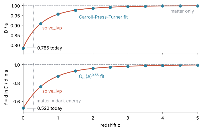
Afterwards you can compute the linear growth factor and growth rate for flat matter plus constant-w dark energy with solve_ivp and check two standard fits.
- Field
- Physics
- Prerequisites
- Cosmological distances with quad: why the farthest galaxies look larger, solve_ivp from the ground up: the pendulum beyond small angles
- Libraries
matplotlib 3.11.2numpy 2.4.3scipy 1.18.1
py-growth-factor.ipynb, executed with the versions above. The download needs a free account
Run it yourself. In a terminal, this installs exactly the versions above:
pip install numpy==2.4.3 scipy==1.18.1 matplotlib==3.11.2 jupyterlabThe problem
You want the linear growth factor \(D(a)\), the factor by which every small density contrast \(\delta = \delta\rho/\rho\) has grown, and the growth rate \(f = d\ln D/d\ln a\), how fast it grows now. Both come from the growth equation, integrated with solve_ivp:
Here \(a = 1/(1+z)\) is the size of the universe relative to today at redshift \(z\), \(H = H_0E(a)\) the expansion rate (\(H_0\) cancels), and a prime is \(d/d\ln a\). \(\Omega_m\) and \(\Omega_\Lambda = 1 - \Omega_m\) are today's shares of matter and dark energy in a flat universe, \(\Omega_m(a)\) the matter share at \(a\), and \(w\) the dark energy's pressure over its density, \(-1\) for Einstein's \(\Lambda\). The \(D'\) term is Hubble drag, the right side self-gravity: matter alone gives \(D = a\), and dark energy lets the drag win. The example is \(\Omega_m = 0.31\), \(w = -1\); swap in your own.
The code
import numpy as np
import matplotlib.pyplot as plt
from scipy.integrate import solve_ivp

# ---- cosmology: replace these with your own
Om = 0.31                  # matter today
OL = 1 - Om                # dark energy today; flat
w = -1.0                   # dark energy pressure / density; -1 is Lambda
a_start = 1e-3             # matter era of this model, which has no radiation

# ---- model: y = [D, dD/dlna], clock lna = ln a
# E2 and dlnH_dlna are the only places the cosmology lives; dlnH_dlna = (1/2) dln(E2)/dlna
def E2(a):
    return Om * a**-3 + OL * a ** (-3 * (1 + w))

def dlnH_dlna(a):
    return -1.5 * (Om * a**-3 + (1 + w) * OL * a ** (-3 * (1 + w))) / E2(a)

def Om_a(a):
    return Om * a**-3 / E2(a)

def growth(lna, y):
    a = np.exp(lna)
    D, dD = y
    return [dD, -(2 + dlnH_dlna(a)) * dD + 1.5 * Om_a(a) * D]

# ---- integrate: growing mode D = a, so dD/dlna = D at the start
sol = solve_ivp(growth, (np.log(a_start), 0.0), [a_start, a_start],
                rtol=1e-10, atol=1e-13, dense_output=True)
z = np.linspace(0, 5, 501)
a = 1 / (1 + z)
D, dD = sol.sol(np.log(a))
f = dD / D

# ---- fits: Carroll, Press, and Turner (1992) for D/a; Linder (2005) for f
def cpt(a):
    m = Om_a(a)
    return 2.5 * m / (m ** (4 / 7) - (1 - m) + (1 + m / 2) * (1 + (1 - m) / 70))

dev_D = np.max(np.abs(cpt(a) / (D / a) - 1))
dev_f = np.max(np.abs(Om_a(a) ** 0.55 / f - 1))
z_eq = (Om / OL) ** (1 / (3 * w)) - 1      # matter and dark energy equally dense

# ---- report and plot
print(f"D/a today: {D[0]:.4f} solve_ivp, {cpt(1.0):.4f} Carroll-Press-Turner;  largest deviation for z <= 5: {dev_D:.2%}")
print(f"f today:   {f[0]:.4f} solve_ivp, {Om**0.55:.4f} Omega_m(a)^0.55;      largest deviation for z <= 5: {dev_f:.2%}")
print(f"D(1) = {D[0]:.4f} with D = a early; normalized to D(1) = 1 instead, D/a -> {1 / D[0]:.3f} early (Pitfall 2)")
print(f"matter = dark energy at z = {z_eq:.2f}")

zm = np.arange(0, 5.01, 0.5)               # where the fits are drawn as markers
am = 1 / (1 + zm)
fig, (ax1, ax2) = plt.subplots(2, 1, sharex=True, figsize=(7, 4.4), dpi=110)
ax1.plot(z, D / a, color="#c8553d", lw=1.8)
ax1.plot(zm, cpt(am), "o", ms=6, color="#2a7f9e", clip_on=False)
ax2.plot(z, f, color="#c8553d", lw=1.8)
ax2.plot(zm, Om_a(am) ** 0.55, "o", ms=6, color="#2a7f9e", clip_on=False)
for ax, y0, fit, y_ivp, y_fit in ((ax1, D[0], "Carroll-Press-Turner fit", 0.9, 0.955), (ax2, f[0], "$\\Omega_m(a)^{0.55}$ fit", 0.74, 0.9)):
    ax.axhline(1, color="#8a8f98", ls="--", lw=1)
    ax.axvline(z_eq, color="#8a8f98", ls=":", lw=1)
    ax.spines[["top", "right"]].set_visible(False)
    ax.text(0.55, y_ivp, "solve_ivp", color="#c8553d", va="top")      # direct labels, in the color of their object
    ax.text(1.6, y_fit, fit, color="#2a7f9e", va="top")
    ax.annotate(f"{y0:.3f} today", (0.08, y0), xytext=(z_eq + 0.1, y0), va="center", arrowprops=dict(arrowstyle="-", color="#8a8f98", lw=0.8))
ax1.text(4.9, 0.985, "matter only", color="#8a8f98", ha="right", va="top")
ax2.text(z_eq + 0.08, 0.575, "matter = dark energy", color="#8a8f98", va="bottom")
ax1.set(ylabel="D / a", ylim=(0.76, 1.01))
ax2.set(xlabel="redshift z", ylabel="f = d ln D / d ln a", xlim=(0, 5), ylim=(0.48, 1.02))
fig.align_ylabels()
plt.show()
D/a today: 0.7849 solve_ivp, 0.7840 Carroll-Press-Turner;  largest deviation for z <= 5: 0.11%
f today:   0.5224 solve_ivp, 0.5251 Omega_m(a)^0.55;      largest deviation for z <= 5: 0.52%
D(1) = 0.7849 with D = a early; normalized to D(1) = 1 instead, D/a -> 1.274 early (Pitfall 2)
matter = dark energy at z = 0.31
Free account
The second half of this tutorial needs a free account
Sign in, or create an account with your email address, and the page goes on right here. The account costs nothing and also brings the notebook download, collections, and done marks.
Still to come
- The knobs
- Pitfalls