Cosmological distances with quad: why the farthest galaxies look larger (Python)

The problem: why the farthest galaxies look larger

A galaxy 10 kpc across covers 1.59 arcseconds on the sky at redshift z = 0.5. Move the same galaxy out to z = 1.6 and it shrinks to 1.15″. Move it further, to z = 5.2, and it has grown back to 1.59″. Past a certain redshift, more distant galaxies look larger. The reason is in how cosmological distances work, and the quantity behind it is the angular diameter distance.

In a static universe there is one distance, and it answers every question. In an expanding one the light left the galaxy when everything was closer together, traveled while space grew, and arrives stretched. Each measurement then has its own distance. The angular diameter distance \(d_A\) turns an angle into a size, \(\theta = \text{size}/d_A\). The luminosity distance \(d_L\) turns a measured flux into a luminosity, \(F = L/(4\pi d_L^2)\). The comoving distance \(d_C\) is the separation between the galaxy and us today. Two times come with them: the age of the universe when the light left, and the lookback time, how long the light was under way.

All five are integrals over the expansion rate, and none of them is hard once that rate is written down. The model is flat ΛCDM with two numbers, the expansion rate today and the matter share, valid from today out to z = 10. Each integral is one call to quad, the function from the scipy.integrate tutorial.

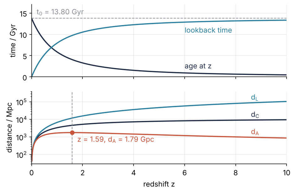
Two panels against redshift z from 0 to 10. Top: age of the universe and lookback time in Gyr, adding up to 13.80 Gyr everywhere. Bottom: comoving, luminosity, and angular diameter distances in Mpc on a log scale; the angular diameter distance peaks at z = 1.59 at 1.79 Gpc and then falls.

The angular diameter distance is the curve that turns over, and its maximum is where the galaxy looks smallest. Step 6 draws the figure.

Setup

ΛCDM is a universe of a cosmological constant Λ plus cold dark matter. Its two parameters are \(H_0\), the expansion rate today, and \(\Omega_m\), the share of today's energy density in matter. Dark energy takes the rest, because the universe is flat: it has no spatial curvature. The cell also prints two scales that Step 1 explains.

import numpy as np
import matplotlib.pyplot as plt
from scipy.integrate import quad
from scipy import constants

plt.rcParams.update({
    "figure.figsize": (7, 3.6), "figure.dpi": 110,
    "axes.spines.top": False, "axes.spines.right": False,
    "axes.grid": True, "grid.alpha": 0.25,
    "font.size": 11, "lines.linewidth": 1.8,
})
INK, ACCENT, SECOND, MUTED = "#1f2a44", "#c8553d", "#2a7f9e", "#8a8f98"

H0 = 67.7                 # km/s/Mpc
Om = 0.31
OL = 1 - Om               # flat

c = constants.c / 1e3                        # km/s
Mpc = 1e6 * constants.parsec / 1e3           # km
Gyr = 1e9 * constants.Julian_year            # s

t_H = Mpc / H0 / Gyr      # Gyr
D_H = c / H0              # Mpc

print(f"t_H = {t_H:.2f} Gyr, D_H = {D_H:.0f} Mpc")

t_H = 14.44 Gyr, D_H = 4428 Mpc

Step 1: Write the expansion rate as a function of redshift

Light that arrives with redshift \(z\) was stretched by the factor \(1 + z\) on the way, and so was everything else: since the light left, the universe has expanded by \(1 + z\), so its size then was \(1/(1 + z)\) of today's. The expansion rate at that time follows from the Friedmann equation, which says that \(H^2\) is proportional to the total energy density. Divide that density by today's and take the root, and \(H(z) = H_0 E(z)\) with

\[E(z) = \sqrt{\Omega_m (1 + z)^3 + \Omega_\Lambda}.\]

The same matter sat in a volume smaller by \((1 + z)^3\), so its density was higher by that factor. Dark energy has the same density at every time, so its term stays constant.

Two scales come out of \(H_0\) alone. The Hubble time \(t_H = 1/H_0\) is how long the universe would have taken to reach its size today at today's rate, and the Hubble distance \(D_H = c/H_0\) is how far light gets in that time. For \(H_0 = 67.7\) km/s/Mpc they are 14.44 Gyr and 4428 Mpc. Setup gets \(t_H\) in Gyr by writing a Mpc in km, which cancels the km/Mpc in \(H_0\) and leaves seconds. The age turns out to be close to \(t_H\), and nothing we see is more than a few \(D_H\) away.

def E(z):
    return np.sqrt(Om * (1 + z) ** 3 + OL)

for z in [0, 1, 10]:
    print(f"z = {z:2d}   E(z) = {E(z):6.3f}")

z =  0   E(z) =  1.000
z =  1   E(z) =  1.780
z = 10   E(z) = 20.330

\(E(0) = 1\) is the check that \(\Omega_m + \Omega_\Lambda = 1\). At \(z = 10\) the universe expanded 20 times faster than today, almost all of it from the matter term.

Step 2: Integrate the age and the lookback time

Write the size of the universe as \(a = 1/(1 + z)\). Its relative growth rate is \(H\), so \(da/a = H\,dt\), and with \(da/a = -dz/(1 + z)\) the time a step \(dz\) takes is \(dz/((1 + z)H)\). Summed from the galaxy's redshift to infinity, the beginning, that is the age at \(z\); summed from 0 to \(z\), it is the lookback time:

\[t(z) = t_H \int_z^\infty \frac{dz'}{(1 + z')E(z')}, \qquad t_L(z) = t_H \int_0^z \frac{dz'}{(1 + z')E(z')}.\]

Today's age \(t_0 = t(0)\) is one quad to infinity. Before building on the integrand, check it: for flat ΛCDM without radiation the age has a closed form, \(t(z) = \frac{2 t_H}{3\sqrt{\Omega_\Lambda}} \operatorname{asinh}\bigl(\sqrt{\Omega_\Lambda/\Omega_m}\,(1 + z)^{-3/2}\bigr)\). If the two agree, the integrand and the units are right.

def dt_dz(z):
    return 1 / ((1 + z) * E(z))

def lookback(z):
    return t_H * quad(dt_dz, 0, z)[0]

def age_exact(z):
    return 2 * t_H / (3 * np.sqrt(OL)) * np.arcsinh(np.sqrt(OL / Om) * (1 + z) ** -1.5)

t0 = t_H * quad(dt_dz, 0, np.inf)[0]
print(f"age today   quad {t0:.4f} Gyr   closed form {age_exact(0):.4f} Gyr"
      f"   difference {abs(t0 - age_exact(0)):.1e} Gyr")
print(f"z = 1       lookback {lookback(1):.2f} Gyr   age then {t0 - lookback(1):.2f} Gyr")

age today   quad 13.7971 Gyr   closed form 13.7971 Gyr   difference 0.0e+00 Gyr
z = 1       lookback 7.94 Gyr   age then 5.86 Gyr

The universe is 13.80 Gyr old, 0.96 \(t_H\), and quad and the closed form agree to the last bit. The infinite upper limit costs nothing extra: quad maps it onto a finite interval, and the integrand falls off as \((1 + z)^{-5/2}\), fast enough that the early universe adds little to the age. Light from \(z = 1\) left 7.94 Gyr ago, when the universe was 5.86 Gyr old. The age at \(z\) needs no second integral: it is \(t_0\) minus the lookback time.

Step 3: Integrate the comoving distance

The comoving distance is the separation today. In each interval \(dt\) light covers \(c\,dt\), and the expansion since then has made that piece of the path \(1 + z\) times longer. The factor \(1 + z\) cancels the one in the time integrand, which leaves

\[d_C(z) = D_H \int_0^z \frac{dz'}{E(z')}.\]

Compare it with the naive distance, the speed of light times the lookback time:

def comoving(z):
    return D_H * quad(lambda zp: 1 / E(zp), 0, z)[0]

light_travel = c * lookback(1) * Gyr / Mpc
print(f"z = 1   comoving {comoving(1):.0f} Mpc   c x lookback {light_travel:.0f} Mpc")
print(f"z = inf comoving {comoving(np.inf):.0f} Mpc = {comoving(np.inf) / D_H:.2f} D_H")

z = 1   comoving 3396 Mpc   c x lookback 2433 Mpc
z = inf comoving 14442 Mpc = 3.26 D_H

The galaxy is 3396 Mpc away today, but light needed only enough time to cover 2433 Mpc, because the part of the path already behind it kept growing. A press release that says "7.9 billion light-years away" has turned the lookback time into a distance. That number is a time; the distance today is 40 % larger.

Without the \(1/(1 + z)\) the integrand falls off only as \((1 + z)^{-3/2}\), so \(d_C\) still grows past \(z = 10\), though toward a finite limit. The integral to infinity is the farthest any light emitted since the beginning can have come from in this model: 14.4 Gpc, or 3.26 \(D_H\), the "few \(D_H\)" of Step 1.

Step 4: Turn it into luminosity and angular diameter distances

The other two distances follow from \(d_C\) by a factor \(1 + z\) each, for a flat universe.

The angle a galaxy covers was set when the light left. The galaxy had the same size then, but the distance between it and us has since grown by \(1 + z\), so it was that much closer: \(d_A = d_C/(1 + z)\).

The flux loses twice. Each photon arrives with its energy lowered by \(1 + z\), and the photons arrive at a rate lowered by \(1 + z\), since the time between two of them is stretched like their wavelength. The flux therefore drops by \((1 + z)^2\) below \(L/(4\pi d_C^2)\), the light spread over a sphere of radius \(d_C\) today, which is \(d_L = (1 + z)\,d_C\). In a curved universe the step from \(d_C\) to \(d_A\) changes, and the Variations give the form.

Take a galaxy 10 kpc across at \(z = 2\):

size = 10e-3                          # Mpc, a galaxy 10 kpc across
z = 2
d_C = comoving(z)
d_L = (1 + z) * d_C
d_A = d_C / (1 + z)
theta = np.degrees(size / d_A) * 3600  # arcsec
print(f"z = {z}   d_C = {d_C:.0f} Mpc   d_L = {d_L:.0f} Mpc   d_A = {d_A:.0f} Mpc")
print(f"        theta = {theta:.2f} arcsec   d_L / d_A = {d_L / d_A:.0f}")

z = 2   d_C = 5311 Mpc   d_L = 15932 Mpc   d_A = 1770 Mpc
        theta = 1.17 arcsec   d_L / d_A = 9

The galaxy covers 1.17″, and its luminosity distance is nine times its angular diameter distance, \((1 + z)^2\) at \(z = 2\). At \(z = 10\) that factor is 121. Both are "the distance to the galaxy", and they differ by two orders of magnitude.

Step 5: Sweep the redshift and find the turnover

Now repeat this on a grid from \(z = 0.01\) to 10 in steps of 0.01. Starting at 0.01 rather than 0 keeps \(d_A\) away from zero, so the angle never divides by it. That is two finite quad calls per redshift, 2000 in all, a fraction of a second. For a grid like this, one call per point is fine. Pitfalls has the case where it is not, and the cell measures two numbers for it: how many integrand calls one quad costs (neval), and how far np.interp on this grid strays from quad halfway between grid points. It also finds where the angle climbs back to its \(z = 0.5\) value.

zs = np.arange(1, 1001) / 100
t_L = np.array([lookback(z) for z in zs])
age = t0 - t_L
d_C = np.array([comoving(z) for z in zs])
d_L = (1 + zs) * d_C
d_A = d_C / (1 + zs)
theta = np.degrees(size / d_A) * 3600

i = np.argmax(d_A)
print(f"turnover   z = {zs[i]:.2f}   d_A = {d_A[i] / 1e3:.2f} Gpc   theta = {theta[i]:.2f} arcsec")
k = i + np.argmax(theta[i:] >= theta[49])        # theta[49] is z = 0.5
print(f"theta back at its z = 0.5 value ({theta[49]:.2f} arcsec) at z = {zs[k]:.2f}")
print(f"largest |age - closed form| on the grid: {np.max(np.abs(age - age_exact(zs))):.1e} Gyr")
z_mid = zs[:-1] + 0.005                          # halfway between grid points, the worst case
interp_err = np.interp(z_mid, zs, d_C) / np.array([comoving(z) for z in z_mid]) - 1
print(f"largest relative error of np.interp on d_C between grid points: {np.max(np.abs(interp_err)):.1e}")
neval = [quad(lambda zp: 1 / E(zp), 0, z, full_output=1)[2]["neval"] for z in zs]
print(f"integrand calls per quad for d_C: {min(neval)} to {max(neval)}, mean {np.mean(neval):.0f}\n")

print("    z   age/Gyr  lookback/Gyr   d_C/Mpc    d_L/Mpc   d_A/Mpc  theta/arcsec")
for z in [0.5, 1, 2, 3, 5, 10]:
    j = round(z * 100) - 1
    print(f"{zs[j]:5.1f}  {age[j]:8.3f}  {t_L[j]:12.3f}  {d_C[j]:8.1f}  {d_L[j]:9.1f}  {d_A[j]:8.1f}  {theta[j]:12.2f}")

turnover   z = 1.59   d_A = 1.79 Gpc   theta = 1.15 arcsec
theta back at its z = 0.5 value (1.59 arcsec) at z = 5.22
largest |age - closed form| on the grid: 6.5e-14 Gyr
largest relative error of np.interp on d_C between grid points: 3.9e-04
integrand calls per quad for d_C: 21 to 105, mean 46

    z   age/Gyr  lookback/Gyr   d_C/Mpc    d_L/Mpc   d_A/Mpc  theta/arcsec
  0.5     8.602         5.195    1946.1     2919.1    1297.4          1.59
  1.0     5.861         7.936    3396.0     6792.1    1698.0          1.21
  2.0     3.284        10.513    5310.6    15931.8    1770.2          1.17
  3.0     2.149        11.648    6508.1    26032.5    1627.0          1.27
  5.0     1.175        12.622    7952.9    47717.3    1325.5          1.56
 10.0     0.474        13.323    9646.5   106111.8     877.0          2.35

The angular diameter distance peaks at \(z = 1.59\), at 1.79 Gpc, where the galaxy covers 1.15″. Up to there, a more distant galaxy looks smaller, as you would expect. Beyond it, the comoving distance still grows, but more slowly than \(1 + z\), so \(d_A\) falls. \(d_A\) is the distance when the light left, and beyond the turnover the universe was so much smaller then that a more distant galaxy was closer to us at emission. By \(z = 5.22\) it covers 1.59″ again, as much as at \(z = 0.5\). The age along the whole grid matches the closed form to 1e-13 Gyr. At \(z = 10\) the universe was under half a billion years old.

Step 6: Plot the times and the distances

Two panels that share the redshift axis: the times on top, the three distances below on a log scale, with the maximum of \(d_A\) marked.

fig, (ax1, ax2) = plt.subplots(2, 1, sharex=True, figsize=(7, 4.4))
ax1.plot(zs, age, color=INK)
ax1.plot(zs, t_L, color=SECOND)
ax1.axhline(t0, color=MUTED, lw=1, ls="--")
ax1.text(0.2, t0 + 0.9, rf"$\mathregular{{t_0}}$ = {t0:.2f} Gyr", color=MUTED)
ax1.text(6.0, 10.4, "lookback time", color=SECOND)
ax1.text(6.0, 2.0, "age at z", color=INK)
ax1.set(ylabel="time / Gyr", ylim=(0, 17))

ax2.semilogy(zs, d_C, color=INK)
ax2.semilogy(zs, d_L, color=SECOND)
ax2.semilogy(zs, d_A, color=ACCENT)
ax2.axvline(zs[i], color=MUTED, lw=1, ls="--")
ax2.plot(zs[i], d_A[i], "o", color=ACCENT, ms=6)
ax2.text(zs[i] + 0.2, d_A[i] * 0.3, rf"z = {zs[i]:.2f}, $\mathregular{{d_A}}$ = {d_A[i] / 1e3:.2f} Gpc", color=ACCENT)
for d, name, color in [(d_L, "L", SECOND), (d_C, "C", INK), (d_A, "A", ACCENT)]:
    ax2.text(8.6, d[859] * 1.5, rf"$\mathregular{{d_{name}}}$", color=color)        # just above each curve at z = 8.6
ax2.set(xlabel="redshift z", ylabel="distance / Mpc", xlim=(0, 10), ylim=(30, 4e5))
plt.show()

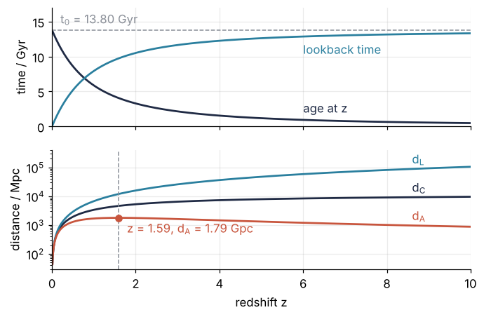
Two panels against redshift z from 0 to 10. Top: age of the universe and lookback time in Gyr, adding up to 13.80 Gyr everywhere. Bottom: comoving, luminosity, and angular diameter distances in Mpc on a log scale; the angular diameter distance peaks at z = 1.59 at 1.79 Gpc and then falls.

The two times add up to \(t_0\) at every redshift, mirror images about half the age. In the lower panel \(d_C\) and \(d_L\) climb all the way to \(z = 10\), while \(d_A\) rises, turns over at the marked point, and falls back to 877 Mpc.

Pitfalls

The luminosity distance for an angular size. A galaxy 10 kpc across at \(z = 2\) comes out at 0.13″ instead of 1.17″, and no turnover appears, because \(d_L\) only grows. The cause is using \(d_L\) where \(d_A\) belongs, often because a paper or a catalog column just says "distance". The rule has no exceptions: sizes with \(d_A\), fluxes with \(d_L\). Keep the subscript in every variable name, so the code says which distance it holds.

Units of Mpc/h mixed with Mpc. Distances come out off by a factor of \(1/h = 1.48\). Simulations and many galaxy catalogs quote lengths in Mpc/h, with \(h = H_0/(100\ \text{km/s/Mpc})\), so that their numbers do not depend on the value of \(H_0\) someone adopts later. Multiplied with distances in plain Mpc, they are wrong by that factor without any error message. Convert once, where the data come in, and put the unit in the variable name, d_C_Mpc_h against d_C_Mpc.

One quad call per galaxy. A mock catalog of a hundred million galaxies from a simulation takes most of an hour. Each call evaluates a Python integrand 21 to 105 times (neval, from the prerequisite), 46 on average over Step 5's grid, about 30 µs per call on the machine that ran this notebook, which is nothing for the 2000 calls of the sweep in Step 5 and everything for a catalog. Tabulate \(d_C\) once on the grid of Step 5, then np.interp(z_catalog, zs, d_C) gives every galaxy at once. On the 0.01 grid, linear interpolation is good to four parts in ten thousand, as the last check of Step 5 shows, which is far better than any photometric redshift. cumulative_trapezoid from scipy.integrate builds the same table in one call.

Variations

A curved universe. Add \(\Omega_k(1 + z)^2\) to \(E(z)^2\), with \(\Omega_k = 1 - \Omega_m - \Omega_\Lambda\), and before dividing by \(1 + z\) replace \(d_C\) by \(D_H \sinh(\sqrt{\Omega_k}\,d_C/D_H)/\sqrt{\Omega_k}\), or the same with \(\sin\) and \(\sqrt{-\Omega_k}\) for \(\Omega_k < 0\) (Hogg 1999).
Radiation, for the early universe. Add \(\Omega_r(1 + z)^4\) with \(\Omega_r \approx 9 \times 10^{-5}\). It changes the age at \(z = 10\) by under half a percent but the age near \(z = 1000\) by about a fifth, and the closed form no longer applies.
Dark energy that evolves. Replace \(\Omega_\Lambda\) by \(\Omega_\Lambda(1 + z)^{3(1 + w)}\) for a constant equation of state \(w\), the ratio of pressure to energy density; \(w = -1\) is Λ.
Check against astropy. astropy.cosmology.FlatLambdaCDM(H0=67.7, Om0=0.31) leaves radiation out by default (Tcmb0=0), and its age, lookback_time, comoving_distance, and angular_diameter_distance reproduce Steps 2 to 5.

Cheat sheet

from scipy.integrate import quad, cumulative_trapezoid           # Om, H0, c, Mpc, Gyr as in Setup
E = lambda z: np.sqrt(Om * (1 + z)**3 + 1 - Om)                  # flat ΛCDM, H(z) = H0 E(z)
t_H, D_H = Mpc / H0 / Gyr, c / H0                                # Gyr, Mpc (Mpc in km, Gyr in s, c in km/s)
t0 = t_H * quad(lambda x: 1 / ((1 + x) * E(x)), 0, np.inf)[0]    # age today
t_L = lambda z: t_H * quad(lambda x: 1 / ((1 + x) * E(x)), 0, z)[0]   # lookback; age at z = t0 - t_L(z)
d_C = lambda z: D_H * quad(lambda x: 1 / E(x), 0, z)[0]          # comoving: separation today
d_L, d_A = lambda z: (1 + z) * d_C(z), lambda z: d_C(z) / (1 + z)     # fluxes with d_L, sizes with d_A
z_grid = np.linspace(0, 10, 1001)                                # many galaxies: tabulate once
d_C_grid = D_H * cumulative_trapezoid(1 / E(z_grid), z_grid, initial=0)
d_C_cat = np.interp(z_catalog, z_grid, d_C_grid)                 # z_catalog: your array of redshifts