Laser rate equations with solve_ivp: relaxation oscillations at turn-on

The problem

Switch a semiconductor laser to 1.5 times its threshold current and the light arrives late, in spikes that ring down. You want this transient from the laser rate equations with solve_ivp, its ringing frequency and damping checked against the small-signal formula. The carriers \(N\) in the active region and the photons \(S\) in the cavity obey

with \(I/q\) the electrons injected per second, \(\tau_n\) and \(\tau_p\) the carrier and photon lifetimes, \(G_N\) the gain per carrier above transparency \(N_\text{tr}\), the carrier number of zero gain, and \(\beta\) the share of spontaneous emission into the lasing mode, seeding the first photons. At threshold gain equals loss, and without \(\beta\) the photon number stands still:

Linearized about the steady state \((N_s, S_s)\), the Jacobian's characteristic equation (stiffness) is a damped oscillator's:

The lifetimes differ by a factor of 1,000, so the cell compares three solvers' nfev to test whether that makes it stiff. Swap in your own laser.

The code

Copy

import numpy as np
import matplotlib.pyplot as plt
from scipy.constants import e as q
from scipy.integrate import solve_ivp

# ---- laser, a typical bulk InGaAsP one: replace with your own
tau_p, tau_n = 2e-12, 2e-9          # photon and carrier lifetimes, s
G_N, N_tr, beta = 1e4, 1e8, 1e-4    # gain per carrier (1/s), transparency, spontaneous share
N_th = N_tr + 1 / (G_N * tau_p)     # gain equals loss
I_th = q * N_th / tau_n
I = 1.5 * I_th
print(f"I_th = {I_th*1e3:.1f} mA, I = {I*1e3:.1f} mA")

# ---- model: y = [N, S], carriers in the active region and photons in the cavity
def rhs(t, y):
    N, S = y
    stim = G_N * (N - N_tr) * S
    return [I / q - N / tau_n - stim, stim - S / tau_p + beta * N / tau_n]
def peak(t, y):                     # dS/dt falls through zero at every spike maximum
    return rhs(t, y)[1]
peak.direction = -1

# ---- integrate: does the factor 1,000 between the lifetimes make it stiff?
for method in ["RK45", "Radau", "LSODA"]:     # sol keeps the LSODA run
    sol = solve_ivp(rhs, (0, 20e-9), [0, 0], method=method, events=peak,
                    dense_output=True, rtol=1e-8, atol=1e-6)
    print(f"{method:6s} {sol.nfev:7,d} nfev {sol.t.size - 1:6,d} steps")

# ---- measure; window on the peak excess: see The knobs
N_s, S_s = sol.y[:, -1]             # the last point: the run must have settled
tp, Sp = sol.t_events[0], sol.y_events[0][:, 1]
ex = Sp / S_s - 1
win = (ex > 1e-3) & (ex < 0.1)
f_meas = 1 / np.diff(tp[win]).mean()
slope, icpt = np.polyfit(tp[win], np.log(ex[win]), 1)
print(f"first spike {Sp[0]:,.0f} photons at {tp[0]*1e9:.2f} ns ({Sp[0]/S_s:.1f} S_s), "
      f"first spacing {(tp[1]-tp[0])*1e9:.2f} ns\n{win.sum()} peaks in window, last excess {ex[-1]:.1e}")

# ---- small-signal formula
wR2 = G_N * S_s / tau_p
Gam = 0.5 * (1 / tau_n + G_N * S_s + beta * N_s / (tau_n * S_s))
f_form = np.sqrt(wR2 - Gam**2) / (2 * np.pi)
print(f"f / GHz        measured {f_meas/1e9:.3f}   formula {f_form/1e9:.3f}")
print(f"Gamma / 1e8/s  measured {-slope/1e8:.2f}    formula {Gam/1e8:.2f} "
      f"({0.5 * (1 / tau_n + G_N * S_s) / 1e8:.2f} without beta)")

# ---- plot: filled markers are the peaks in the window
t = np.linspace(0.05e-9, 15e-9, 6000)
fig, (a1, a2) = plt.subplots(2, 1, sharex=True, figsize=(7, 4.6), dpi=110)
a1.semilogy(t * 1e9, sol.sol(t)[1], color="#c8553d", lw=1.6)
a1.axhline(S_s, color="#2a7f9e", ls="--", lw=1)
a1.text(14.9, S_s / 2.5, "steady state", color="#2a7f9e", ha="right", va="top")
a1.text(tp[0] * 1e9, 1.4e6, f"{Sp[0]:,.0f} at {tp[0]*1e9:.2f} ns", color="#c8553d")
a1.set(ylim=(1, 1e7), ylabel="photons in the cavity")
a2.semilogy(tp * 1e9, np.exp(icpt) * np.exp(-Gam * tp), color="#2a7f9e", lw=1.2)
a2.set(xlim=(0, 15), ylim=(3e-4, 10), xlabel="t / ns", ylabel="$S_{peak}/S_s - 1$")
for a, y, c in [(a1, Sp, "#c8553d"), (a2, ex, "#c8553d")]:
    a.plot(tp * 1e9, y, "o", color=c, ms=4, mfc="white"); a.plot(tp[win] * 1e9, y[win], "o", color=c, ms=4)
    a.spines[["top", "right"]].set_visible(False); a.grid(alpha=0.25)
plt.show()

I_th = 12.0 mA, I = 18.0 mA
RK45    14,750 nfev  2,260 steps
Radau   34,090 nfev  4,515 steps
LSODA    5,956 nfev  4,234 steps
first spike 403,025 photons at 2.41 ns (5.4 S_s), first spacing 0.38 ns
21 peaks in window, last excess 1.8e-05
f / GHz        measured 3.081   formula 3.081
Gamma / 1e8/s  measured 6.79    formula 6.75 (6.25 without beta)

The knobs

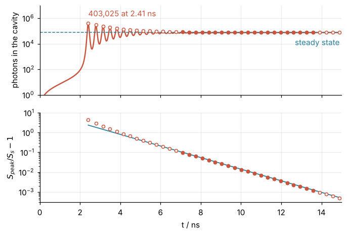
The pump sets the steady state. Above threshold the carriers stay clamped near \(N_\text{th}\) and every further electron leaves as a photon, so \(S_s/\tau_p \approx (I - I_\text{th})/q\) and \(\omega_R^2 \approx G_N (I - I_\text{th})/q\): the frequency grows as \(\sqrt{I/I_\text{th} - 1}\), and \(\Gamma\) grows with \(S_s\), so a harder pump rings faster and settles sooner. \(\tau_p\) and \(G_N\) set the threshold, and \(G_N\) the frequency once more. \(\tau_n\) sets the delay: while \(S\) is still tiny, \(N\) charges toward \(I\tau_n/q\) with time constant \(\tau_n\) and passes \(N_\text{th}\) after \(\tau_n \ln[I/(I - I_\text{th})] = 2\ \text{ns} \times \ln 3 = 2.20\) ns, and the first spike follows 0.21 ns later. \(N_s\) and \(S_s\) are the last point of the run, so the run must have settled. The 20 ns span 13.6 damping times \(1/\Gamma\), and the last peak's excess is down to 1.8 × 10⁻⁵. A weaker pump or a smaller \(G_N\) damps more slowly, so lengthen the run until that excess sits far below the window's lower edge: a wrong \(S_s\) shifts every excess and spoils the fit and the formula alike.

rtol sets how far down the window may reach. It bounds the error of each step, but a late peak carries what thousands of the run's 4,234 steps have piled up, many times rtol. The edge at \(10^{-3}\) keeps all 21 fitted excesses far above that. Before you lower it, tighten rtol tenfold and check that the fitted \(\Gamma\) stays put. The \(\beta\) term lifts the formula's \(\Gamma\) from 6.25 to 6.75 × 10⁸ s⁻¹, 8 % more, and the measured 6.79 × 10⁸ s⁻¹ sides with it. That \(\Gamma\) is exact, half the trace of the Jacobian, while \(\omega_R^2\) drops three small terms, each carrying \(\beta\). In the lower panel the line takes the formula's slope and the fit's intercept, so its height agrees by construction and its slope is the test. The measured \(f\) is the ringing frequency, equal to \(\omega_R/2\pi\) only while \(\Gamma \ll \omega_R\) (here \(\omega_R\) is nearly 30 times \(\Gamma\)), so for a strongly damped laser compare against \(f\). The log axis shows the photons climbing out of spontaneous emission during the delay, which a linear one flattens to zero. What the output does not mean: this is a single-mode model with linear gain. Real diode lasers saturate the gain, which damps the spikes faster, and add side modes and heating.

Pitfalls

No spontaneous emission term. Set beta = 0 and the laser never lights. With \(S(0) = 0\) the photon equation gives \(dS/dt = 0\) at every instant, so \(S\) stays at zero for all 20 ns while \(N\) settles at \(I\tau_n/q = 1.5\,N_\text{th}\). Above threshold that is an unstable equilibrium, and nothing in the equations kicks the laser out of it. Keep the \(\beta N/\tau_n\) term rather than starting from \(S = 1\), which lights the laser but drops the term from the damping.

Radau by reflex. A factor of 1,000 between the lifetimes looks like stiffness, so the implicit Radau seems the safe choice. The counts say otherwise: Radau reports an nfev of 34,090, 2.3 times the 14,750 of RK45, and that leaves out the calls it spends on its finite-difference Jacobian; LSODA, whose count includes them, reports 5,956. In the terms of the stiffness tutorial, the system is stiff only before the light comes on: while the carriers are below transparency, the photon equation has an eigenvalue of magnitude at least \(1/\tau_p\) = 5 × 10¹¹ s⁻¹. Above threshold the coupling turns the two eigenvalues into \(-\Gamma \pm i\,2\pi f\), of magnitude about 2 × 10¹⁰ s⁻¹, a scale any solver must resolve anyway to follow the ringing. Compare nfev before you choose, as the cell does, and use LSODA, which switches to an implicit method only where it pays.

Fitting the first spikes. The first spikes are large-signal: the first reaches 5.4 times \(S_s\), far outside any linearization, and they come slower. The first spacing, 0.38 ns, is a frequency of 2.6 GHz, 15 % below the 3.081 GHz of the ringing. Fit all peaks, or start with the first two, and both the frequency and the damping come out wrong. Keep the window on the peak excess between \(10^{-3}\) and 0.1, as in the code, so that only spikes within 10 % of \(S_s\) count; the figure fills their markers.