Stiffness: why an explicit solver crawls on a reaction that has long settled (Python)

The question

The Robertson reaction, proposed by H. H. Robertson in 1966, is three species and three reactions, and it is the classic test of stiffness. A turns into B with a rate constant of 0.04 s⁻¹. Two molecules of B meet and one of them becomes C, with a rate constant of 3 × 10⁷. B meets C and turns back into A, with 10⁴. The last two reactions are second order, so their constants are per unit concentration per second, and every concentration here is scaled by the initial concentration of A, which starts alone: \(y = (1, 0, 0)\). The fastest constant is 7.5 × 10⁸ times the slowest. Mass action gives the rate equations

\[ \begin{aligned} y_A' &= -0.04\, y_A + 10^4\, y_B\, y_C, \\ y_B' &= \phantom{-}0.04\, y_A - 10^4\, y_B\, y_C - 3 \times 10^7\, y_B^2, \\ y_C' &= 3 \times 10^7\, y_B^2 . \end{aligned} \]

Here they are integrated over 40 s with solve_ivp, once with its default method, RK45, and once with Radau, both at rtol=1e-6, atol=1e-10:

Show code

import numpy as np
import matplotlib.pyplot as plt
from scipy.integrate import solve_ivp

plt.rcParams.update({
    "figure.figsize": (7, 3.6), "figure.dpi": 110,
    "axes.spines.top": False, "axes.spines.right": False,
    "axes.grid": True, "grid.alpha": 0.25,
    "font.size": 11, "lines.linewidth": 1.8,
})
INK, ACCENT, SECOND, MUTED = "#1f2a44", "#c8553d", "#2a7f9e", "#8a8f98"

k1, k2, k3 = 0.04, 3e7, 1e4      # 1/s; k2 and k3 per unit of scaled concentration

def robertson(t, y):
    A, B, C = y
    return [-k1 * A + k3 * B * C,
            k1 * A - k3 * B * C - k2 * B**2,
            k2 * B**2]

y0, t_span = [1.0, 0.0, 0.0], (0, 40)
tol = dict(rtol=1e-6, atol=1e-10)
rk45 = solve_ivp(robertson, t_span, y0, method="RK45", **tol)
radau = solve_ivp(robertson, t_span, y0, method="Radau", dense_output=True, **tol)

for name, s in [("RK45", rk45), ("Radau", radau)]:
    print(f"{name:5s} {s.nfev:8,d} calls {len(s.t) - 1:7,d} steps   mean step {np.diff(s.t).mean() * 1e3:6.1f} ms   "
          f"at 40 s: A = {s.y[0, -1]:.4f}  B = {s.y[1, -1]:.3e}  C = {s.y[2, -1]:.4f}")

t = np.logspace(-6, np.log10(40), 400)
A, B, C = radau.sol(t)
fig, ax = plt.subplots()
for curve in [A, 1e4 * B, C]:                    # one color: all three are the reference solution
    ax.semilogx(t, curve, color=INK)
ax.text(2e-6, 0.93, "A", color=INK, va="top")
ax.text(25, 0.34, "C", color=INK, ha="center")
ax.text(4.6e-3, 0.40, "B × 10⁴", color=INK, ha="center")
ax.set(xlabel="t / s", ylabel="concentration / initial A", xlim=(1e-6, 40), ylim=(0, 1.05))
plt.show()

RK45   242,066 calls  34,537 steps   mean step    1.2 ms   at 40 s: A = 0.7158  B = 9.185e-06  C = 0.2842
Radau      647 calls      78 steps   mean step  512.8 ms   at 40 s: A = 0.7158  B = 9.186e-06  C = 0.2842

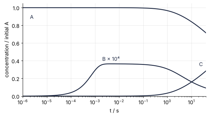
Concentrations of A, B (times 10⁴), and C in the Robertson reaction against time on a log axis from 1 µs to 40 s. B jumps to its plateau within the first few milliseconds; A and C change only over seconds.

The intermediate B shoots up in the first few milliseconds, peaks at 3.6 × 10⁻⁵ after 4.6 ms, and from then on sinks slowly. A and C barely move until about 0.1 s and then drift over seconds. Once B has peaked, nothing in this picture changes faster than on a scale of seconds, and the two methods agree on A and C at 40 s to four digits.

Yet RK45 needed 242,066 calls of the right-hand side in 34,537 steps, a mean step of 1.2 ms, all the way to 40 s. Radau needed 647 calls in 78 steps, a factor of 374 fewer calls. The solve_ivp tutorial names stiffness in its pitfalls and tells you to switch methods. The question here is why: why does a solver that controls its own error crawl in millisecond steps along a curve a ruler could follow, and why does Radau not have to?

The idea: a step that overshoots a curve it should land on

Look at what B does. Once it has peaked, any deviation from the level that the current A and C allow dies out in about half a millisecond, far faster than that level moves, and B is carried along by the slow change of A. Strip that to one variable and you get a version of the test equation of Curtiss and Hirschfelder (1952),

\[y' = -1000\,(y - \cos t),\]

with the 1000 in the role of B's fast relaxation and \(\cos t\) in the role of the slow drift. Whatever \(y\) starts at, it is pulled toward \(\cos t\) with a time constant of 1/1000 s, and within a few milliseconds every solution has fallen onto the slow curve and stays there. That curve is itself an exact solution, \(\cos t\) shifted by about \(0.001 \sin t\), and the distances below are measured from it.

Explicit Euler, the simplest solver, takes the slope at the point where it stands and follows it for one step \(h\). On the slow curve that slope is gentle. A little off the curve it is steep, because the 1000 multiplies the distance to the curve. If the step is shorter than about the time constant, following that steep slope brings the solution toward the curve. If it is longer, the step carries the solution past the curve to the other side, and the next slope is steep in the opposite direction. Here are three step sizes, starting from \(y(0) = 0.5\), with neighboring exact solutions drawn faintly so that you can see how steep the slopes are off the curve:

lam = -1000.0                                    # 1/s: the fast relaxation onto the slow curve

def f(t, y):
    return lam * (y - np.cos(t))

def slow(t):
    # the solution the others fall onto: cos t, shifted by about 0.001 sin t
    return (lam**2 * np.cos(t) - lam * np.sin(t)) / (lam**2 + 1)

def exact(t, t0, y_start):
    return slow(t) + (y_start - slow(t0)) * np.exp(lam * (t - t0))

def explicit_euler(h, t_end, y_start):
    t = h * np.arange(round(t_end / h) + 1)
    y = np.empty_like(t)
    y[0] = y_start
    for n in range(len(t) - 1):
        y[n + 1] = y[n] + h * f(t[n], y[n])     # the slope where you stand
    return t, y

steps = [0.0008, 0.0019, 0.0021]                 # s
fig, axes = plt.subplots(3, 1, figsize=(7, 6.3), sharex=True)
for ax, h in zip(axes, steps):
    for t0 in np.arange(0, 0.05, 0.0025):
        tt = np.linspace(t0, t0 + 0.005, 40)
        for ys in [0.0, 0.4, 1.6, 2.0]:
            ax.plot(tt, exact(tt, t0, ys), color=MUTED, lw=0.7, alpha=0.5)
    t_fine = np.linspace(0, 0.055, 300)
    ax.plot(t_fine, slow(t_fine), color=INK)
    t_e, y_e = explicit_euler(h, 0.05, 0.5)
    ax.plot(t_e, y_e, "o-", color=ACCENT, ms=4, lw=1)
    ax.text(0.01, 0.97, f"h = {h * 1e3:.1f} ms   1 + hλ = {1 + h * lam:+.1f}".replace("-", "−"),
            transform=ax.transAxes, va="top")
    ax.set(ylim=(-0.2, 2.9), yticks=[0, 1, 2], ylabel="y")
axes[-1].set(xlabel="t / s", xlim=(-0.001, 0.052))
plt.show()

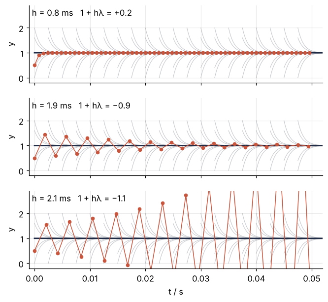
Explicit Euler on y′ = −1000 (y − cos t) at three step sizes, y against t up to 0.05 s. At 0.8 ms the points approach the slow curve; at 1.9 ms they zigzag across it and settle; at 2.1 ms the zigzag grows.

At 0.8 ms the points slide onto the curve and stay on it. At 1.9 ms they zigzag across it, and the zigzag dies out. At 2.1 ms the zigzag grows with every step and leaves the panel.

The factor behind this comes from one Euler step. Since both \(y\) and the slow curve solve the same linear equation, the distance between them, \(e\), obeys \(e' = \lambda e\) with \(\lambda = -1000\) s⁻¹. The curve barely bends within a step, so one step turns \(e\) into \(e + h\lambda e = (1 + h\lambda)\, e\). When \(1 + h\lambda\) lies between 0 and 1, the distance shrinks. Between −1 and 0, it changes sign and shrinks: the zigzag that dies out. Below −1, which happens for \(h > 2/1000\) s, every step throws the solution across the curve to a point further away than where it started:

print(" h / ms   1 + hλ   off the curve at 0.05 s   at 1 s")
for h in steps:
    off = [abs(y[-1] - slow(t[-1])) for t, y in (explicit_euler(h, T, 0.5) for T in (0.05, 1.0))]
    print(f"{h * 1e3:6.1f}   {1 + h * lam:+5.1f}   {off[0]:20.1e}   {off[1]:8.1e}")

 h / ms   1 + hλ   off the curve at 0.05 s   at 1 s
   0.8    +0.2                4.0e-07    2.2e-07
   1.9    -0.9                3.2e-02    5.1e-07
   2.1    -1.1                4.9e+00    2.5e+19

A factor of −0.9 and a factor of −1.1 look alike, and they are worlds apart: after 1 s the run at 1.9 ms is off the slow curve by 5.1 × 10⁻⁷, and the run at 2.1 ms by 2.5 × 10¹⁹. Nothing about \(\cos t\) changed between the two. The step limit is set by the 1000, the process that finished in the first few milliseconds, not by the curve you are following.

The implicit step: take the slope where you land

Implicit Euler takes the slope at the end of the step instead of the start:

\[y_{n+1} = y_n + h\, f(t_{n+1}, y_{n+1}).\]

The unknown \(y_{n+1}\) now appears on both sides, so every step is an equation to solve. For the test equation it is linear and can be solved by hand. In terms of the distance from the curve, one step multiplies \(e\) by \(1/(1 - h\lambda)\), which for negative \(\lambda\) lies between 0 and 1 at any \(h\). If the solution is off the curve, the slope at the landing point points back toward the curve, so the step can only pull the solution in. Here it is at \(h = 0.1\) s, fifty times the explicit limit:

def implicit_euler(h, t_end, y_start):
    t = h * np.arange(round(t_end / h) + 1)
    y = np.empty_like(t)
    y[0] = y_start
    for n in range(len(t) - 1):
        # y[n+1] = y[n] + h * lam * (y[n+1] - cos t[n+1]), solved for y[n+1]
        y[n + 1] = (y[n] - h * lam * np.cos(t[n + 1])) / (1 - h * lam)
    return t, y

h = 0.1
t_i, y_i = implicit_euler(h, 1.5, 0.5)
print(f"implicit Euler, h = {h} s: factor 1/(1 - hλ) = {1 / (1 - h * lam):.4f}, "
      f"off the curve after one step {abs(y_i[1] - slow(t_i[1])):.1e}, at 1.5 s {abs(y_i[-1] - slow(t_i[-1])):.1e}")
print(f"explicit Euler at the same h: factor 1 + hλ = {1 + h * lam:+.0f}")

t_fine = np.linspace(0, 1.5, 300)
fig, ax = plt.subplots()
ax.plot(t_fine, slow(t_fine), color=INK)
ax.plot(t_i, y_i, "o", color=SECOND, ms=6)
ax.text(0.98, 0.95, "explicit Euler at this step: 1 + hλ = −99",
        transform=ax.transAxes, ha="right", va="top", color=ACCENT)
ax.set(xlabel="t / s", ylabel="y", ylim=(0, 1.1))
plt.show()

implicit Euler, h = 0.1 s: factor 1/(1 - hλ) = 0.0099, off the curve after one step 5.0e-03, at 1.5 s 5.3e-06
explicit Euler at the same h: factor 1 + hλ = -99

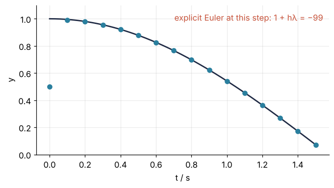
Implicit Euler at a step of 0.1 s, 50 times the explicit limit, on y′ = −1000 (y − cos t) from 0 to 1.5 s, starting at 0.5. After the first step all 15 points lie on the slow curve y = cos t.

One step takes the start at 0.5 to within 5 × 10⁻³ of the curve, and at 1.5 s the 15 steps are off by 5.3 × 10⁻⁶. Explicit Euler at the same step would multiply every deviation by −99.

Watch both methods side by side at the same step of 2.1 ms, just above the explicit limit. Each step draws the slope its method uses, then the point it lands on:

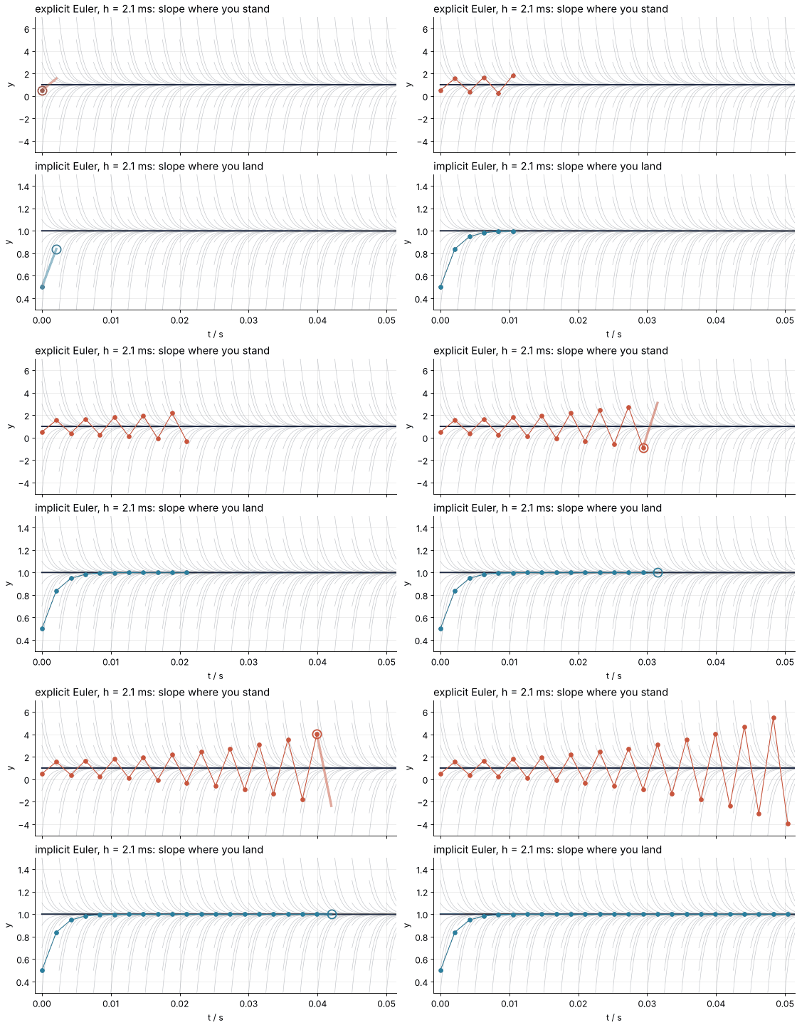
Animation of explicit and implicit Euler at the same 2.1 ms step on y′ = −1000 (y − cos t). Each step draws its slope, then its new point. The explicit points zigzag ever further across the curve; the implicit points land on it within four steps.

How I built this: Matplotlib animation with FuncAnimation: a probe sweep as a small GIF.

The price is the equation in every step. Here it was one line of algebra. For Robertson, or any nonlinear system, it is a system of nonlinear equations at every step, and the formalization says what solving it costs.

Formalization

Near a solution of \(y' = f(t, y)\), a small deviation \(\delta\) obeys \(\delta' = J\,\delta\), where \(J = \partial f / \partial y\) is the Jacobian, the matrix of partial derivatives of each component of \(f\) with respect to each component of \(y\). Each eigenvalue \(\lambda\) of \(J\) is a mode that grows or decays like \(e^{\lambda t}\), so \(1/|\mathrm{Re}\,\lambda|\) is a time scale. A problem is stiff when some of its modes decay far faster than the solution you are following changes: the fast modes have died out, and their eigenvalues are still there. The test is the fastest time scale against the span you integrate over.

For Robertson the Jacobian is read off the rate equations above, and its eigenvalues, computed with NumPy, change along the solution:

def robertson_jac(t, y):
    A, B, C = y
    return np.array([[-k1,  k3 * C,               k3 * B],
                     [ k1, -k3 * C - 2 * k2 * B, -k3 * B],
                     [0.0,  2 * k2 * B,           0.0]])

print("  t / s       eigenvalues of J / (1/s)          fast time    slow time")
for t in [1e-4, 1e-2, 1, 40]:
    ev = np.sort(np.linalg.eigvals(robertson_jac(t, radau.sol(t))).real)
    print(f"{t:7.0e}   {ev[0]:9.1f} {ev[1]:9.4f} {ev[2]:9.1e}   {1e3 / abs(ev[0]):6.2f} ms   {1 / abs(ev[1]):6.1f} s")

  t / s       eigenvalues of J / (1/s)          fast time    slow time
  1e-04      -239.0   -0.0799  -3.9e-17     4.18 ms     12.5 s
  1e-02     -2190.3   -0.4039  -4.4e-17     0.46 ms      2.5 s
  1e+00     -2179.6   -0.2941  -4.4e-16     0.46 ms      3.4 s
  4e+01     -3392.8   -0.0214  -2.2e-16     0.29 ms     46.7 s

At 40 s the fast eigenvalue is −3,393 s⁻¹, a time scale of 0.29 ms against a span of 40 s and a slow time scale of 47 s. The ratio is 1.6 × 10⁵. The third eigenvalue is zero up to rounding: A + B + C is conserved, and a deviation along it neither grows nor decays.

The stability region. Explicit Euler multiplies a deviation by \(1 + h\lambda\) per step and is stable when \(|1 + h\lambda| \le 1\), a disk of radius 1 around −1 in the complex plane of \(h\lambda\). A Runge-Kutta method such as RK45 takes several slopes per step instead of one: the slope at the start, then the slope at a trial point a fraction of the step ahead, then at a trial point built from both, and so on. These intermediate slopes are the stages, and a table of weights says how much of each goes into the next trial point and into the step. RK45 evaluates six per attempted step, the last at the new point, where it doubles as the first slope of the next step. Applied to \(y' = \lambda y\), each slope is \(\lambda\) times its trial point, so each trial point is \(y\) plus \(h\lambda\) times a weighted sum of earlier ones, so the whole step multiplies \(y\) by a polynomial \(R(h\lambda)\), here evaluated from SciPy's own weights:

Show code

from scipy.integrate import RK45
from scipy.optimize import brentq

A_rk = np.zeros((6, 6))
A_rk[:, :5] = RK45.A                             # SciPy's weights, padded to a square table

def R_rk45(z):
    """Factor by which one RK45 step multiplies y on y' = λy, with z = hλ."""
    z = np.asarray(z, dtype=complex)
    stages = []
    for i in range(6):                           # each stage uses the slopes of the earlier ones
        stages.append(1 + z * sum(A_rk[i, j] * stages[j] for j in range(i)))
    return 1 + z * sum(RK45.B[i] * stages[i] for i in range(6))

z_limit = brentq(lambda x: abs(R_rk45(x)) - 1, -4, -2.5)
attempts = (rk45.nfev - 2) // 6                  # two calls to start, six per attempted step
print(f"RK45 is stable on the negative real axis down to hλ = {z_limit:.2f}")
print(f"RK45 on Robertson: {attempts:,d} attempted steps, {len(rk45.t) - 1:,d} accepted, "
      f"{attempts - (len(rk45.t) - 1):,d} rejected")

x, y = np.meshgrid(np.linspace(-5, 3, 801), np.linspace(-3.6, 3.6, 721))
z = x + 1j * y
fig, ax = plt.subplots(figsize=(6, 4.4))
ax.contourf(x, y, (abs(R_rk45(z)) <= 1).astype(float), levels=[0.5, 1.5], colors=[ACCENT], alpha=0.30)
ax.contourf(x, y, (abs(1 + z) <= 1).astype(float), levels=[0.5, 1.5], colors=[ACCENT], alpha=0.35)
ax.contour(x, y, abs(1 + z), levels=[1], colors=[ACCENT], linewidths=1.2)
ax.contour(x, y, abs(1 - z), levels=[1], colors=[SECOND], linewidths=1.6)
ax.axvline(0, color=MUTED, ls="--", lw=1)
ax.plot(z_limit, 0, "o", color=ACCENT, ms=6)
ax.annotate(f"RK45 limit {z_limit:.2f}".replace("-", "−"), (z_limit, 0), xytext=(-4.9, -2.6), color=ACCENT,
            arrowprops=dict(arrowstyle="-", color=ACCENT, lw=0.8))
ax.text(-1, -1.15, "explicit Euler", color=ACCENT, ha="center", va="top")
ax.text(-2.4, 1.9, "RK45", color=ACCENT, ha="center")
ax.text(1, 1.15, "implicit Euler:\nstable outside", color=SECOND, ha="center", va="bottom")
ax.text(-4.9, 3.1, "decaying modes", color=MUTED, va="top")
ax.text(0.15, -3.1, "growing", color=MUTED, va="bottom")
ax.set(xlabel="Re hλ", ylabel="Im hλ", aspect="equal", xlim=(-5, 3), ylim=(-3.3, 3.3))
plt.show()

RK45 is stable on the negative real axis down to hλ = -3.31
RK45 on Robertson: 40,344 attempted steps, 34,537 accepted, 5,807 rejected

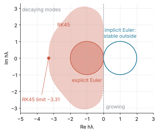
Stability regions in the complex plane of h times λ. Explicit Euler: a disk of radius 1 around −1. RK45: a larger bounded region reaching −3.31 on the real axis. Implicit Euler: stable everywhere outside a disk around +1, so on the whole left half.

RK45's region is larger than Euler's but bounded, and on the negative real axis it ends at \(h\lambda = -3.31\). On Robertson at 40 s that allows \(h = 3.31/3393 = 0.98\) ms, which is the step RK45 is taking. Every explicit method has a bounded region, and for a Runge-Kutta method the reason is that a polynomial grows without limit far enough out. Implicit Euler's factor \(1/(1 - h\lambda)\) has modulus below 1 for every \(\lambda\) with negative real part, a property called A-stability. So does the factor of Radau IIA, the method behind method="Radau".

Accuracy and stability are separate limits, and the solver only watches accuracy. RK45 estimates the error of each step and rejects a step whose error is too large. A step beyond the bound makes the fast mode grow, the error estimate sees it, the step is rejected and shrunk, and the next steps creep back up until one fails again. That is why the steps hover at \(3.31/|\lambda|\) instead of staying below it. At six calls per attempt, plus two at the start for the first slope and the choice of the first step, the 242,066 calls are 40,344 attempts for 34,537 accepted steps: 5,807 steps were thrown away.

The price of implicit: the Jacobian and a linear solve. Each implicit step solves a nonlinear system by Newton's method, which turns it into a few linear systems with matrices \(I - h\gamma J\), \(\gamma\) a fixed number of the method (\(\gamma = 1\) for implicit Euler). Each such matrix is factored once, an LU factorization, and reused for every solve while \(h\) and \(J\) stay about the same. On Robertson, Radau evaluated 18 Jacobians (the counter njev) and made 100 factorizations (nlu). For three species that is free. For hundreds of species it is the cost that matters, and passing jac, the Jacobian as a function, or jac_sparsity, the pattern of nonzero entries of a large and mostly empty \(J\), keeps it down.

SciPy's documentation gives the rule of thumb. Start with RK45. If it takes unusually many steps, diverges, or fails, the problem is most likely stiff: switch to Radau or BDF, or to LSODA, which detects stiffness and switches methods by itself. BDF, the backward differentiation formulas, is implicit Euler built on the last few points instead of one, and more points raise its order, the power of \(h\) with which the error over a fixed span shrinks. SciPy's BDF varies the order from 1 to 5. On large systems I try BDF first: it factors one matrix per update, Radau two, one of them complex. Do not assume it is A-stable: only orders 1 and 2 are, so for modes that oscillate more than they decay, with eigenvalues near the imaginary axis, take Radau.

See it in code

The first Radau run, in the opening cell, had no Jacobian and approximated \(J\) by finite differences, calls of the right-hand side that nfev does not count. The cell gives the implicit methods the analytic Jacobian from above, so that every call they make is in the count, solves Robertson with all four methods, and then computes the fast eigenvalue at every RK45 step. A solver taking steps of length \(h\) makes \(1/h\) steps per second, so the total number of steps is the integral of \(1/h\) over time, and with \(h = 3.31/|\lambda_\text{fast}|\) that integral predicts how many steps RK45 must take:

Show code

runs = {}
print("method      calls   Jacobians   LU   steps")
for method in ["RK45", "Radau", "BDF", "LSODA"]:
    extra = {} if method == "RK45" else {"jac": robertson_jac}
    s = runs[method] = solve_ivp(robertson, t_span, y0, method=method, **tol, **extra)
    print(f"{method:6s} {s.nfev:10,d} {s.njev:11d} {s.nlu:4d} {len(s.t) - 1:7,d}")

s = runs["RK45"]
J = np.array([robertson_jac(t, y) for t, y in zip(s.t, s.y.T)])    # shape (n, 3, 3)
lam_fast = np.abs(np.linalg.eigvals(J)).max(axis=1)              # eigvals works on a stack of matrices
bound = abs(z_limit) / lam_fast
predicted = np.trapezoid(1 / bound, s.t)
h_rk = np.diff(s.t)
after = s.t[:-1] > 1e-2
ratio = h_rk[after] / bound[:-1][after]
print(f"\nRK45 steps predicted from the fast eigenvalue: {predicted:,.0f}, taken: {len(s.t) - 1:,d}")
print(f"after 10 ms, RK45 steps from {h_rk[after].min() * 1e3:.2f} to {h_rk[after].max() * 1e3:.2f} ms, "
      f"h|λ_fast| median {abs(z_limit) * np.median(ratio):.2f}, mean {abs(z_limit) * ratio.mean():.2f}")
h_rd = np.diff(runs["Radau"].t)
print(f"Radau steps from {h_rd.min() * 1e3:.2f} ms to {h_rd.max():.1f} s")

fig, ax = plt.subplots(figsize=(7, 4))
ax.loglog(s.t[:-1], h_rk, ".", color=ACCENT, ms=2, alpha=0.6, rasterized=True)
ax.loglog(s.t, bound, color=MUTED, ls="--", lw=1.2, zorder=3)
ax.loglog(runs["Radau"].t[:-1], h_rd, "o", color=SECOND, ms=4)
ax.text(2e-2, 2.5e-3, "RK45", color=ACCENT)
ax.text(3, 0.08, "Radau", color=SECOND)
ax.text(2e-2, 4.5e-4, r"$3.31\,/\,|\lambda_\mathrm{fast}|$", color=MUTED)
ax.text(0.02, 0.95, f"RK45 steps predicted {predicted:,.0f}, taken {len(s.t) - 1:,d}",
        transform=ax.transAxes, va="top")
ax.set(xlabel="t / s", ylabel="step h / s", xlim=(1e-6, 40), ylim=(5e-5, 20))
plt.show()

method      calls   Jacobians   LU   steps
RK45      242,066           0    0  34,537
Radau         647          18  100      78
BDF           366           4   33     144
LSODA         330          28   28     200

RK45 steps predicted from the fast eigenvalue: 34,568, taken: 34,537
after 10 ms, RK45 steps from 0.79 to 1.71 ms, h|λ_fast| median 3.25, mean 3.31
Radau steps from 0.08 ms to 3.3 s

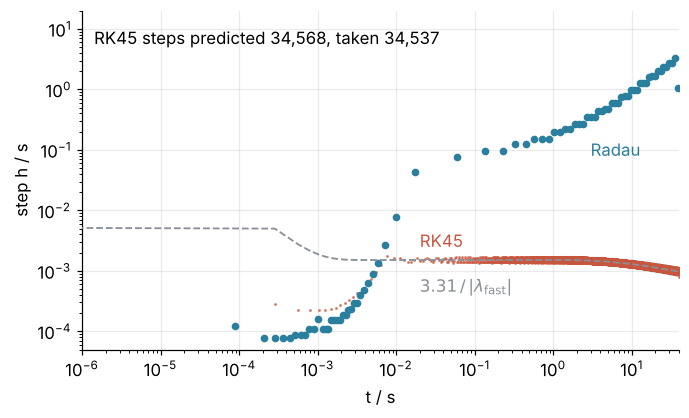
Step size against time on log-log axes along the Robertson solution. RK45 steps climb to the dashed bound 3.31 over the fast eigenvalue by 10 ms and follow it to 40 s, between 0.8 and 1.7 ms; Radau steps grow from 0.08 ms to 3.3 s. Predicted 34,568 RK45 steps, taken 34,537.

Radau made 647 calls, as many as in the first run, so the finite-difference calls there had indeed gone uncounted; here the rest of the work is 18 calls of robertson_jac. BDF and LSODA, the other two choices of the rule of thumb, finish in 366 and 330 calls. The prediction from the eigenvalue alone is 34,568 steps against 34,537 taken, within 0.1 %. After the first 10 ms RK45's steps, between 0.79 and 1.71 ms, scatter around the dashed bound, with \(h|\lambda_\text{fast}|\) at a median of 3.25 and a mean of 3.31, while Radau's steps grow from 0.08 ms to 3.3 s, more than four orders of magnitude. The cost of an explicit solver on a stiff problem is set by the eigenvalue of a mode that died out in the first milliseconds.

Where it shows up

Combustion. Detailed mechanisms such as GRI-Mech 3.0, with 53 species and 325 reactions for natural gas, contain radicals that equilibrate far faster than the flame they feed. Cantera integrates its reactor networks with CVODES from SUNDIALS, an implicit BDF code.
Atmospheric chemistry. Photochemical mechanisms for ozone mix short-lived radicals with species that persist for years. Chemical transport models generate Rosenbrock solvers for them with the Kinetic PreProcessor, KPP, which writes the Jacobian and its sparsity pattern into the code.
Electrical circuits. A parasitic capacitance of picofarads in a circuit whose interesting behavior takes milliseconds makes a stiff system. SPICE integrates with the implicit trapezoidal rule or Gear's backward differentiation formulas, the ancestors of BDF.
Chemical engineering. Reactor models with fast equilibria, acid-base or adsorption, next to slow conversion are stiff for the same reason Robertson is. They are often written as differential-algebraic systems, with the fast equilibria replaced by algebraic equations, and integrated by implicit codes such as IDA from SUNDIALS.
Partial differential equations. The heat equation discretized on a grid by the method of lines has a fast eigenvalue near \(-4D/\Delta x^2\). That gives explicit Euler a step limit of \(\Delta x^2/(2D)\) on a line, so ten times finer in space costs a hundred times more steps in time, and py-pde from the ground up: the heat equation on a square plate runs into the same limit on its grid.

In every case a fast process that has finished still sets the step of an explicit method, and the fast eigenvalue tells you how small.

The question

The idea: a step that overshoots a curve it should land on

The implicit step: take the slope where you land

Formalization

See it in code

Where it shows up

Further reading