Linear programming with scipy.optimize.linprog: the cheapest cement blend

The problem: the cheapest raw meal for a cement kiln

A cement kiln is fed a powder ground from four materials: limestone, clay, sand, and iron ore. The kiln needs the lime (CaO), silica (SiO2), and iron oxide (Fe2O3) of the blend each inside a narrow window. Limestone costs 3.5 EUR per tonne and iron ore 40, so the question is which mix meets all three windows for the least money. The answer is 4.80 EUR per tonne, and finding it is a linear program, solved by one call to scipy.optimize.linprog.

The prices and contents in this tutorial are invented, in the range of a real raw meal. Lime and silica combine in the kiln into the minerals of the clinker, and the iron oxide helps the mix melt. Too little or too much of any of them spoils the clinker, so each has a lower and an upper limit.

The oxide content of a blend is the average of the materials' contents, weighted by their mass fractions, and its cost is the same weighted average of the prices. With \(x_j\) the fraction of material \(j\), \(c_j\) its price, and \(a_{kj}\) its content of oxide \(k\) in percent, the task is

\[\min_x \sum_j c_j x_j \quad\text{subject to}\quad \ell_k \le \sum_j a_{kj} x_j \le u_k, \qquad \sum_j x_j = 1, \qquad x_j \ge 0,\]

where \(\ell_k\) and \(u_k\) are the limits of the window for oxide \(k\). Every term is a fraction times a constant. That is what makes it linear.

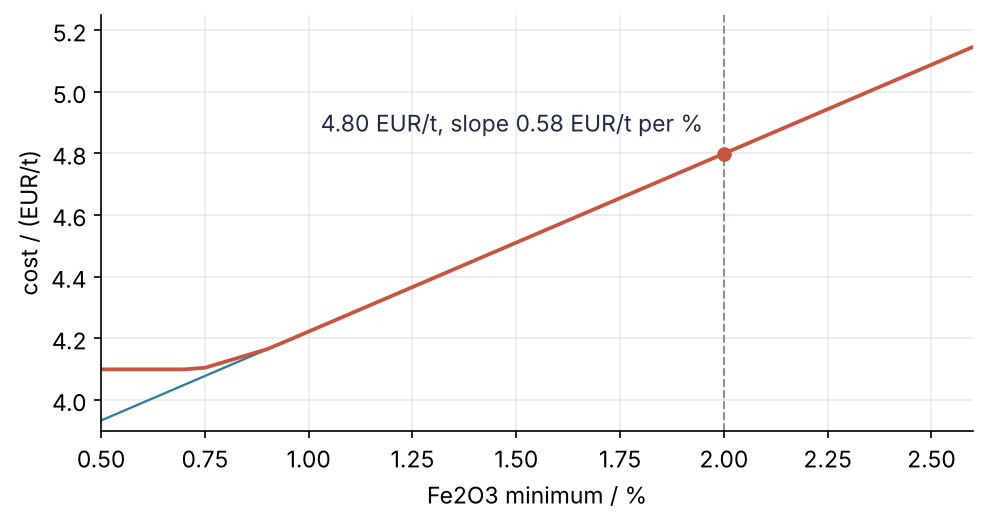
Lowest cost of the raw meal, in EUR per tonne, against the Fe2O3 minimum of the specification, 0.5 to 2.6 %. The cost is flat, then rises in two straight pieces. At the plant's 2.0 % a dot marks 4.80 EUR/t, and a thin line with the dual-value slope, 0.58 EUR/t per %, lies on the curve from 0.90 % up and runs below it to the left.

This is where we end up: the cheapest cost as a function of how much iron oxide the specification demands. At the plant's 2.0 % each further percentage point costs 0.58 EUR per tonne, a number linprog hands you without being asked. Step 4 draws the figure from 43 solves.

Setup

One cell: imports, the look of the figures, and the data. The tables are the place for your own materials and limits. Nothing in this tutorial is random, so there is nothing to seed.

import numpy as np
import matplotlib.pyplot as plt
from scipy.optimize import linprog

plt.rcParams.update({
    "figure.figsize": (7.5, 3.6), "figure.dpi": 110,
    "axes.spines.top": False, "axes.spines.right": False,
    "axes.grid": True, "grid.alpha": 0.25,
    "font.size": 11, "lines.linewidth": 1.8,
})
INK, ACCENT, SECOND, MUTED = "#1f2a44", "#c8553d", "#2a7f9e", "#8a8f98"

# ---- your own data: replace these tables
names = ["limestone", "clay", "sand", "iron ore"]
cost = np.array([3.5, 9.0, 7.0, 40.0])             # EUR per tonne
oxides = ["CaO", "SiO2", "Fe2O3"]
content = np.array([[51.0,  2.0,  0.5,  3.0],      # mass percent, one row per oxide
                    [ 4.0, 58.0, 92.0, 12.0],
                    [ 0.4,  6.0,  0.8, 62.0]])
lo = np.array([42.0, 13.5, 2.0])                   # specification window, percent
hi = np.array([44.0, 14.5, 2.6])

print(f"{'':10s}" + "".join(f"{n:>10s}" for n in names))
print(f"{'EUR/t':10s}" + "".join(f"{v:10.1f}" for v in cost))
for ox, row, l, h in zip(oxides, content, lo, hi):
    print(f"{ox + ' / %':10s}" + "".join(f"{v:10.1f}" for v in row) + f"    window {l:.1f} to {h:.1f}")

           limestone      clay      sand  iron ore
EUR/t            3.5       9.0       7.0      40.0
CaO / %         51.0       2.0       0.5       3.0    window 42.0 to 44.0
SiO2 / %         4.0      58.0      92.0      12.0    window 13.5 to 14.5
Fe2O3 / %        0.4       6.0       0.8      62.0    window 2.0 to 2.6

Step 1: Write the blend as matrices

linprog solves one shape of problem: minimize c @ x subject to A_ub @ x <= b_ub, A_eq @ x == b_eq, and bounds on each variable. The price list is c as it stands. An oxide window has two sides, but A_ub holds only upper limits, so each window becomes two rows. The upper limit goes in as it is, content @ x <= hi. The lower limit, content @ x >= lo, is multiplied by −1 on both sides, which turns the inequality around: -content @ x <= -lo.

That the fractions sum to one is an equality, and A_eq exists for it. Two inequalities, at most one and at least one, would say the same with more signs to get wrong. bounds=(0, 1) applies to every fraction at once; a list of pairs, one per material, sets them one by one.

A_ub = np.vstack([content, -content])     # three upper limits, then the three lower ones flipped
b_ub = np.concatenate([hi, -lo])
A_eq = np.ones((1, 4))                    # the fractions sum to one
b_eq = [1.0]
labels = [f"{ox} max" for ox in oxides] + [f"{ox} min" for ox in oxides]

for label, row, b in zip(labels, A_ub, b_ub):
    print(f"{label:9s} [" + " ".join(f"{a:6.1f}" for a in row) + f" ] @ x <= {b:6.1f}")

CaO max   [  51.0    2.0    0.5    3.0 ] @ x <=   44.0
SiO2 max  [   4.0   58.0   92.0   12.0 ] @ x <=   14.5
Fe2O3 max [   0.4    6.0    0.8   62.0 ] @ x <=    2.6
CaO min   [ -51.0   -2.0   -0.5   -3.0 ] @ x <=  -42.0
SiO2 min  [  -4.0  -58.0  -92.0  -12.0 ] @ x <=  -13.5
Fe2O3 min [  -0.4   -6.0   -0.8  -62.0 ] @ x <=   -2.0

The bottom three rows carry minus signs on both sides: the −13.5 on the right of the SiO2 row is how linprog hears "at least 13.5 %".

Seen as geometry, four fractions that sum to one leave three free directions, and the blends with no negative fraction fill a tetrahedron whose corners are the four pure materials. Each row is a flat cut through it, each window keeps the slab between two parallel cuts, and what survives all six cuts is the allowed region, a solid with flat faces. A linear cost falls steadily in one direction, so its lowest point in such a solid is a corner, where at least three limits are met exactly. A bound \(x_j \ge 0\) is a limit too, met when material \(j\) is left out. So if the cheapest blend uses all four materials, at least three oxide limits must be met exactly: the active limits.

Step 2: Solve and read the result

res = linprog(cost, A_ub=A_ub, b_ub=b_ub, A_eq=A_eq, b_eq=b_eq, bounds=(0, 1), method="highs")
print(res.status, res.message)
for name, frac in zip(names, res.x):
    print(f"{name:10s} {100 * frac:6.2f} %")
print(f"cost       {res.fun:6.2f} EUR/t")
for ox, val, l, h in zip(oxides, content @ res.x, lo, hi):
    print(f"{ox:6s} {val:6.2f} %   window {l:.1f} to {h:.1f}")

0 Optimization terminated successfully. (HiGHS Status 7: Optimal)
limestone   85.93 %
clay         3.17 %
sand         8.65 %
iron ore     2.25 %
cost         4.80 EUR/t
CaO     44.00 %   window 42.0 to 44.0
SiO2    13.50 %   window 13.5 to 14.5
Fe2O3    2.00 %   window 2.0 to 2.6

Status 0 means an optimum was found; with any other value res.x is not your answer, as the pitfalls show. All four materials are in, 85.93 % of it limestone, and the blend costs 4.80 EUR per tonne. The last three lines are the check to make every time: CaO sits at its 44.0 % maximum, SiO2 and Fe2O3 at their minimums of 13.5 and 2.0 %. Three active limits, as the corner count predicted. The cheap limestone goes in as far as the CaO ceiling allows, and the expensive iron ore only as far as the iron minimum forces.

method="highs" is the default. It hands the problem to the HiGHS solver and picks between "highs-ds", a simplex method that walks from corner to corner of the allowed region, and "highs-ipm", an interior point method that cuts through its inside. On this problem both return the same blend. The older "simplex", "revised simplex", and "interior-point" still run but warn that they are deprecated. Do not use them.

Step 3: Find the limits that hold the optimum

res.ineqlin holds two arrays with one entry per row of A_ub. residual is the slack, how far the blend is from that row's limit, b_ub - A_ub @ x; it is zero for an active limit. marginals is the dual value of each row, also called its shadow price: the change in res.fun per unit increase of that row's b_ub. The rows are in percent, so a marginal is in EUR per tonne per percentage point.

The sign needs one thought. Every row is an upper limit, so raising its b_ub loosens it, and a looser limit can only make the cheapest blend cheaper: the marginals are zero or negative. For a minimum row, raising b_ub = -lo lowers the minimum, which loosens it too: the SiO2 row's −13.5 raised to −13.4 reads "at least 13.4 %". Either way, minus the marginal is what it costs to make that limit one point stricter:

print(f"{'limit':9s} {'slack / %':>9s}   cost of one point stricter / (EUR/t)")
# + 0.0 turns a rounded -0.0 into 0.0, so no "-0.0000" is printed
for label, slack, marginal in zip(labels, res.ineqlin.residual, res.ineqlin.marginals):
    print(f"{label:9s} {round(slack, 2) + 0.0:9.2f}   {round(-marginal, 4) + 0.0:8.4f}")

limit     slack / %   cost of one point stricter / (EUR/t)
CaO max        0.00     0.0144
SiO2 max       1.00     0.0000
Fe2O3 max      0.60     0.0000
CaO min        2.00     0.0000
SiO2 min       0.00     0.0289
Fe2O3 min      0.00     0.5775

Three rows have zero slack, the three active limits from Step 2, and only they have a price. The Fe2O3 minimum costs 0.5775 EUR per tonne per point, the SiO2 minimum 0.0289, the CaO maximum 0.0144. The iron limit is forty times as expensive as the lime limit. The loose rows cost nothing to tighten a little, because the optimum does not touch them.

A marginal is a derivative, so check it the honest way: raise the Fe2O3 minimum to 2.01 % and solve again.

lo_strict = lo + np.array([0, 0, 0.01])
res_strict = linprog(cost, A_ub=A_ub, b_ub=np.concatenate([hi, -lo_strict]),
                     A_eq=A_eq, b_eq=b_eq, bounds=(0, 1))
print(f"cost change per point of Fe2O3: {(res_strict.fun - res.fun) / 0.01:.4f} EUR/t")

cost change per point of Fe2O3: 0.5775 EUR/t

The same 0.5775. res.eqlin.marginals holds the same kind of number for the sum-to-one row, which is not a specification anyone negotiates; leave it alone. A dual value holds only while the same limits stay active. Move the iron minimum far enough and another limit takes over.

Step 4: Sweep the iron specification and draw the cost

Solve once for each Fe2O3 minimum from 0.5 to 2.6 %, 0.05 apart, and print the slope of the cost at three places: the first interval, the seventh (0.80 to 0.85 %), and the last. The slope changes where the active limits change. With a low iron minimum, iron ore at 40 EUR per tonne is the candidate to leave out, and cheap limestone keeps CaO at its maximum. The cell therefore also computes the two blends with no iron ore, CaO at 44.0 %, and SiO2 at one end of its window, three linear equations in three fractions each. Their Fe2O3 content is where to look for the kinks.

fe_min = np.linspace(0.5, 2.6, 43)
fe_cost = np.array([
    linprog(cost, A_ub=A_ub, b_ub=np.concatenate([hi, -np.array([lo[0], lo[1], f])]),
            A_eq=A_eq, b_eq=b_eq, bounds=(0, 1)).fun
    for f in fe_min])
slope = np.diff(fe_cost) / np.diff(fe_min)
print(f"cost {fe_cost[0]:.2f} to {fe_cost[-1]:.2f} EUR/t, "
      f"slopes {round(slope[0], 3) + 0.0:.3f}, {slope[6]:.3f}, {slope[-1]:.4f} EUR/t per %")

no_ore = np.vstack([content[:2, :3], np.ones(3)])    # CaO and SiO2 rows, sum to one, iron ore out
for sio2 in [hi[1], lo[1]]:
    blend = np.linalg.solve(no_ore, [hi[0], sio2, 1.0])
    print(f"CaO 44.0 %, SiO2 {sio2:.1f} %, no iron ore: Fe2O3 {content[2, :3] @ blend:.3f} %")

price_fe = -res.ineqlin.marginals[5]
fig, ax = plt.subplots()
ax.plot(fe_min, res.fun + price_fe * (fe_min - lo[2]), color=SECOND, lw=1.1)   # the dual value as a slope
ax.plot(fe_min, fe_cost, color=ACCENT)
ax.axvline(lo[2], color=MUTED, ls="--", lw=1)
ax.plot(lo[2], res.fun, "o", color=ACCENT, ms=6)
ax.annotate(f"{res.fun:.2f} EUR/t, slope {price_fe:.2f} EUR/t per %", (lo[2], res.fun),
            xytext=(-10, 8), textcoords="offset points", ha="right", va="bottom", color=INK)
ax.set(xlabel="Fe2O3 minimum / %", ylabel="cost / (EUR/t)", xlim=(0.5, 2.6), ylim=(3.9, 5.25))
plt.show()

cost 4.10 to 5.15 EUR/t, slopes 0.000, 0.404, 0.5775 EUR/t per %
CaO 44.0 %, SiO2 14.5 %, no iron ore: Fe2O3 0.737 %
CaO 44.0 %, SiO2 13.5 %, no iron ore: Fe2O3 0.903 %

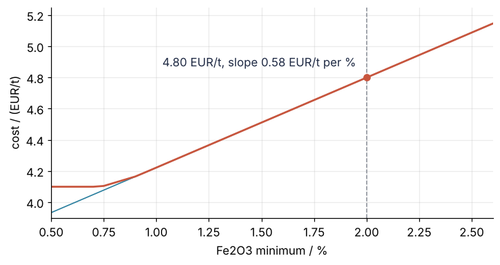
Lowest blend cost in EUR/t against the Fe2O3 minimum, 0.5 to 2.6 %. Flat at 4.10 up to 0.74 %, then two straight rises with a kink at 0.90 %. A dot at 2.0 % marks 4.80 EUR/t; a thin line with the dual-value slope, 0.58 EUR/t per %, follows the curve down to 0.90 % and leaves it below.

Below 0.74 % the cost is flat at 4.10 EUR per tonne. The cheapest blend there is the first of the two: no iron ore, CaO and SiO2 at their maximums, and already 0.737 % Fe2O3, so the iron minimum is not active. From 0.74 % the iron minimum is active and is met by replacing sand with clay, which carries more iron, at 0.404 EUR per tonne per point, while the silica falls from its maximum. At 0.903 %, the second blend, the silica reaches its 13.5 % minimum, and from there only iron ore can supply the iron, at 0.5775 EUR per tonne per point, up to 5.15 EUR per tonne at the 2.6 % ceiling.

The thin line is the dual value from Step 3 as a prediction. It lies on the curve over the whole segment the plant operates on and leaves it at the kink at 0.90 %. Each kink is a move to a neighboring corner of the allowed region, with one active limit traded for another.

Pitfalls

Maximizing without negating. linprog only minimizes. To maximize a profit you pass -profit and negate res.fun. Get the sign wrong and nothing complains: hand the cement problem -cost by mistake and it maximizes the cost.

wrong = linprog(-cost, A_ub=A_ub, b_ub=b_ub, A_eq=A_eq, b_eq=b_eq, bounds=(0, 1))
print(f"status {wrong.status}, cost {-wrong.fun:.2f} EUR/t")

status 0, cost 5.20 EUR/t

Status 0 and 5.20 EUR per tonne: the most expensive blend inside the specification, reported as a success. The same mistake on a profit returns the least profitable plan.

An infeasible specification. An Fe2O3 minimum of 2.8 % above its own 2.6 % maximum is the obvious case. The instructive one is a CaO window of 45 to 46 %, which looks reachable because limestone alone has 51 %. linprog answers only that the problem is infeasible. To find the conflict, drop the two CaO rows and ask how much CaO the remaining limits allow at most. That is another linear program: maximize the CaO content by minimizing -content[0], the negation from the pitfall above, once with the silica and iron rows together and once with each alone. A set of rows whose highest CaO stays below 45 % is the culprit.

b_hot = np.concatenate([[46.0, hi[1], hi[2]], [-45.0, -lo[1], -lo[2]]])
res_hot = linprog(cost, A_ub=A_ub, b_ub=b_hot, A_eq=A_eq, b_eq=b_eq, bounds=(0, 1))
print(res_hot.status, res_hot.success, res_hot.x)
print(res_hot.message)

# rows 0 and 3 are the CaO limits; keep only the ones listed
for rows, kept in [([1, 2, 4, 5], "SiO2 and Fe2O3"), ([1, 4], "SiO2 only"), ([2, 5], "Fe2O3 only")]:
    r = linprog(-content[0], A_ub=A_ub[rows], b_ub=b_ub[rows], A_eq=A_eq, b_eq=b_eq, bounds=(0, 1))
    blend = ", ".join(f"{n} {round(100 * v, 1) + 0.0:.1f} %" for n, v in zip(names, r.x))
    print(f"{kept:15s} highest CaO {-r.fun:5.2f} %   ({blend})")

2 False None
The problem is infeasible. (HiGHS Status 8: model_status is Infeasible; primal_status is None)
SiO2 and Fe2O3  highest CaO 44.45 %   (limestone 86.9 %, clay 0.0 %, sand 10.6 %, iron ore 2.5 %)
SiO2 only       highest CaO 45.55 %   (limestone 89.2 %, clay 0.0 %, sand 10.8 %, iron ore 0.0 %)
Fe2O3 only      highest CaO 49.75 %   (limestone 97.4 %, clay 0.0 %, sand 0.0 %, iron ore 2.6 %)

Status 2, res.x is None, and the message names no culprit. The silica and iron windows together allow at most 44.45 % CaO: meeting both minimums takes 10.6 % sand and 2.5 % iron ore, which carry almost no CaO and dilute it. The silica window alone allows 45.55 %, the iron window alone 49.75 %, so only the pair conflicts. Check res.status before you read res.x. Once you know the conflicting pair, widen one of its windows or add a material.

Units mixed between rows. Write the Fe2O3 row in mass fractions (0.62 for iron ore) while its limits stay in percent (2.0), and the row can never reach its minimum: linprog reports the problem infeasible. With other numbers the mix-up gives a wrong answer and status 0. Keep a row and its limits in one unit, and print content @ res.x next to lo and hi as Step 2 does.

Variations

A supply limit on one material. Per-variable bounds: bounds=[(0, 1), (0, 0.25), (0, 1), (0, 1)] caps clay at 25 %.
A ratio between oxides. CaO / SiO2 at most 3.2 becomes, multiplied out, CaO − 3.2 SiO2 ≤ 0: one more row content[0] - 3.2 * content[1] in A_ub with 0 in b_ub.
Whole truckloads or on/off decisions. The integrality= argument of linprog makes HiGHS solve a mixed-integer program, a linear program with some variables restricted to whole numbers; scipy.optimize.milp is the full interface for those. The matrices stay the same.
Many products and many plants. Transport and production planning use the same three arrays, larger and mostly zeros; A_ub may then be a scipy.sparse matrix.

Cheat sheet

res = linprog(c, A_ub=A_ub, b_ub=b_ub,        # rows of A_ub @ x <= b_ub
              A_eq=A_eq, b_eq=b_eq,           # rows of A_eq @ x == b_eq
              bounds=(0, None),               # one pair for all, or a list of pairs
              method="highs")                 # the default; "highs-ds", "highs-ipm"
# a row a @ x >= b goes in as -a @ x <= -b
if res.status != 0: print(res.message)        # 2 infeasible, 3 unbounded
res.x, res.fun                                # the optimum and its cost
res.ineqlin.residual                          # slack per row; 0 means the limit is active
-res.ineqlin.marginals                        # cost of tightening each row by one unit
res = linprog(-profit, ...); best = -res.fun   # to maximize, minimize the negative