Minimization with scipy.optimize.minimize: the shape of a seven-atom cluster

The problem: the shape of seven argon atoms

Put seven argon atoms in a box, cool them down, and they settle into the arrangement of lowest energy. That arrangement is a pentagonal bipyramid, a ring of five atoms with one above and one below, at an energy of −16.505 ε. Finding it is one call to scipy.optimize.minimize, or rather, as you will see, fifty calls, because most single calls end at −15.533 ε instead.

Two atoms at distance \(r\) interact through the Lennard-Jones potential

\[V(r) = 4\varepsilon\left[\left(\frac{\sigma}{r}\right)^{12} - \left(\frac{\sigma}{r}\right)^{6}\right],\]

with a well of depth \(\varepsilon\) at \(r = 2^{1/6}\sigma\). We work in reduced units, \(\varepsilon = \sigma = 1\); for argon \(\varepsilon/k_B \approx 120\) K and \(\sigma \approx 3.4\) Å, so one length unit is 3.4 Å. The total energy is the sum of \(V\) over all 21 pairs, a function of 21 coordinates. That function has several minima, and a minimizer walks downhill from its start and stops in the first one it reaches. Which one that is depends on the start and, as Step 4 shows, on the method.

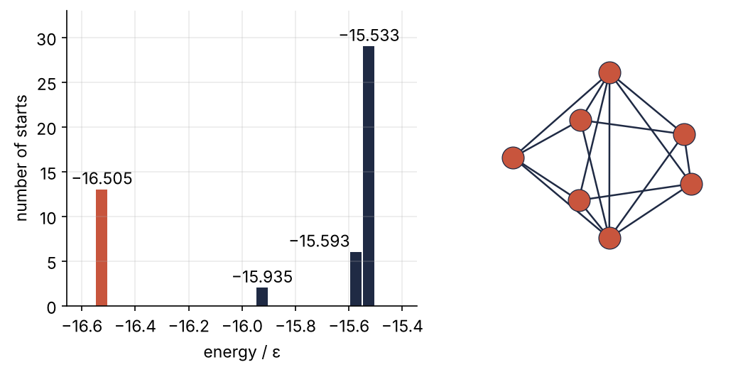
Left: how many of fifty random starts ended at each energy; the leftmost bar, at −16.505 ε, is the global minimum. Right: that structure, a pentagonal bipyramid of seven atoms, drawn without axes because the coordinates of a free cluster carry no meaning.

Each of the fifty starts is one minimize call, and Step 6 draws the result. Most stop at −15.533 ε, and a quarter find the bipyramid.

Setup

The random starting positions are this tutorial's only data. They come from a seeded generator (Random numbers with numpy.random explains default_rng):

import numpy as np
import matplotlib.pyplot as plt
from scipy.optimize import minimize, approx_fprime
from scipy.spatial.distance import pdist, squareform

plt.rcParams.update({
    "figure.figsize": (8, 3.6), "figure.dpi": 110,
    "axes.spines.top": False, "axes.spines.right": False,
    "axes.grid": True, "grid.alpha": 0.25,
    "font.size": 11, "lines.linewidth": 1.8,
})
INK, ACCENT, SECOND, MUTED = "#1f2a44", "#c8553d", "#2a7f9e", "#8a8f98"

rng = np.random.default_rng(1)

def random_start(n, side=2.0, d_min=0.8):
    """n atoms uniform in a cube, as one flat array of 3n coordinates."""
    while True:
        pos = rng.uniform(0, side, size=(n, 3))
        if pdist(pos).min() > d_min:   # no two atoms nearly on top of each other; see Pitfalls
            return pos.ravel()

print(f"pair distance at the bottom of the well: 2^(1/6) = {2 ** (1 / 6):.5f} σ")

pair distance at the bottom of the well: 2^(1/6) = 1.12246 σ

Step 1: Write the energy as a function of one flat array

minimize moves one flat vector of numbers. The physics lives in an array of positions with one row per atom and three columns. The energy function reshapes on the way in, pdist returns the \(n(n-1)/2\) distances between rows, and the sum over pairs is one line:

def energy(x):
    r = pdist(x.reshape(-1, 3))
    return np.sum(4 * (r**-12 - r**-6))

dimer = np.array([0, 0, 0, 2 ** (1 / 6), 0, 0])
x0 = np.array([0, 0, 0, 1.5, 0, 0, 0.3, 1.2, 0])    # three atoms, the start for Step 2
print(f"two atoms at 2^(1/6): E = {energy(dimer):.6f} ε")
print(f"three atoms at x0:    E = {energy(x0):.6f} ε")

two atoms at 2^(1/6): E = -1.000000 ε
three atoms at x0:    E = -1.285777 ε

Two atoms at the bottom of the well give exactly −1, the depth of the pair potential. The function is right. The three-atom start sits at −1.286 ε, the number Step 2 has to improve on.

Step 2: Minimize three atoms and read the result

Hand the function and the start to minimize and print everything it returns:

res = minimize(energy, x0)
print(res)

  message: Optimization terminated successfully.
  success: True
   status: 0
      fun: -2.9999999999999805
        x: [ 3.801e-01 -2.096e-01  9.875e-07  1.238e+00  5.143e-01
             9.654e-07  1.820e-01  8.953e-01 -9.564e-07]
      nit: 19
      jac: [ 1.788e-07 -1.073e-06  0.000e+00  5.364e-07  6.855e-07
             0.000e+00  5.960e-07  1.669e-06  0.000e+00]
 hess_inv: [[ 3.693e-01 -2.704e-02 ... -1.687e-02  2.362e-04]
            [-2.704e-02  3.600e-01 ...  3.501e-01 -2.181e-04]
            ...
            [-1.687e-02  3.501e-01 ...  3.468e-01 -1.001e-04]
            [ 2.362e-04 -2.181e-04 ... -1.001e-04  1.000e+00]]
     nfev: 280
     njev: 28

fun is the energy at the end, −3.0 to fourteen digits. x holds the final coordinates, flat like x0, so reshape it to read positions. success, status, and message say why the minimizer stopped, nit counts its iterations, and nfev counts how often it called your function. jac is the Jacobian, which for a function returning one number is its gradient; at the end every component is below \(2\times10^{-6}\).

With no bounds and no constraints, the default method is BFGS. It follows the slope downhill and builds up a picture of the curvature from the slopes it has seen along the way. The matrix of second derivatives is called the Hessian, and hess_inv is BFGS's estimate of its inverse. BFGS stops and reports success when the largest component of the gradient falls below gtol, by default \(10^{-5}\). So success True means the ground is flat here. It does not mean this is the lowest point, and it does not mean this is the cluster you meant; the last pitfall shows one that is not.

Here it is the lowest point. The three pair distances are all \(2^{1/6}\):

print(pdist(res.x.reshape(-1, 3)))

[1.12246206 1.12246207 1.12246204]

An equilateral triangle, as it should be. The cost is the odd part: 280 function calls for 19 iterations. All of them went into estimating the gradient by finite differences: njev counts 28 estimates, each costing ten calls, one at the point and one per shifted coordinate.

Step 3: Supply the gradient

The gradient of a pair sum follows from the chain rule, for any pair potential. Moving atom \(i\) changes only the distances \(r_{ij}\) to the other atoms, and \(\partial r_{ij}/\partial \mathbf r_i = (\mathbf r_i - \mathbf r_j)/r_{ij}\), so

\[\frac{\partial E}{\partial \mathbf r_i} = \sum_{j \ne i} \frac{V'(r_{ij})}{r_{ij}}\,(\mathbf r_i - \mathbf r_j).\]

For Lennard-Jones in reduced units \(V'(r) = 24 r^{-7} - 48 r^{-13}\), and the factor in the sum is

\[\frac{V'(r)}{r} = 24 r^{-8} - 48 r^{-14}.\]

In code, pos[:, None, :] - pos[None, :, :] broadcasts the positions against themselves into an \(n \times n \times 3\) array d whose entry [i, j] is the vector \(\mathbf r_i - \mathbf r_j\). The diagonal \(i = j\) has distance zero; setting it to infinity makes its factor zero. Summing over the second axis gives one row per atom, and ravel() makes it flat again, the same length as x.

approx_fprime estimates the gradient the way minimize did in Step 2: it moves each coordinate by a tiny step and divides the change in energy by the step. Compare every gradient you write against it. A wrong gradient makes BFGS fail or, worse, stop in the wrong place.

def gradient(x):
    pos = x.reshape(-1, 3)
    d = pos[:, None, :] - pos[None, :, :]
    r = np.linalg.norm(d, axis=2)
    np.fill_diagonal(r, np.inf)          # no self-interaction
    factor = 24 * r**-8 - 48 * r**-14
    return (factor[:, :, None] * d).sum(axis=1).ravel()

x5 = random_start(5)
g = gradient(x5)
print(f"largest difference to approx_fprime: {np.abs(g - approx_fprime(x5, energy)).max() / np.abs(g).max():.1e} of the largest component")

for jac in [None, gradient]:
    r5 = minimize(energy, x5, jac=jac)
    print(f"jac={'gradient' if jac else 'None':8s}  E = {r5.fun:.6f} ε   nfev = {r5.nfev:4d}")

largest difference to approx_fprime: 1.0e-07 of the largest component
jac=None      E = -9.103852 ε   nfev =  976
jac=gradient  E = -9.103852 ε   nfev =   61

Agreement to seven digits, then the same minimum at −9.103852 ε for a sixteenth of the cost: 61 calls instead of 976. The five atoms form a trigonal bipyramid, which the sorted distances show as nine bonds near \(2^{1/6}\) and one long distance, 1.826 σ, between the two apexes:

print(np.sort(pdist(r5.x.reshape(-1, 3))).round(3))

[1.12  1.12  1.12  1.12  1.12  1.12  1.124 1.124 1.124 1.826]

Step 4: Compare methods by their function evaluations

Now seven atoms, one start, four ways to minimize. Two methods are new. Nelder-Mead uses function values only, never a slope: it keeps a simplex of \(n + 1\) points, here 22, and moves it downhill by reflecting, stretching, and shrinking it. L-BFGS-B is BFGS that remembers only the last few steps instead of a full 21 × 21 inverse Hessian, and it can keep variables inside bounds.

x7 = random_start(7)
runs = [("Nelder-Mead", None), ("BFGS", None), ("BFGS", gradient), ("L-BFGS-B", gradient)]
for method, jac in runs:
    r7 = minimize(energy, x7, method=method, jac=jac)
    label = method + (" + gradient" if jac else "")
    print(f"{label:21s} E = {r7.fun:10.6f} ε  success = {r7.success!s:5s}  nfev = {r7.nfev:5d}  {r7.message}")

Nelder-Mead           E = -14.744484 ε  success = False  nfev =  4200  Maximum number of function evaluations has been exceeded.
BFGS                  E = -15.533060 ε  success = True   nfev =  2024  Optimization terminated successfully.
BFGS + gradient       E = -15.533060 ε  success = True   nfev =    89  Optimization terminated successfully.
L-BFGS-B + gradient   E = -16.505384 ε  success = True   nfev =    70  CONVERGENCE: RELATIVE REDUCTION OF F <= FACTR*EPSMCH

Read the last column first. Nelder-Mead stopped at its default limit of 200 calls per variable, 4,200 in all, with success False and an energy that is no minimum at all. In 21 dimensions it is the wrong tool. BFGS needs 2,024 calls without the gradient and 89 with it, a factor of 23, and both land at −15.533 ε.

L-BFGS-B, from the same start, reaches −16.505 ε in 70 calls. That is the luck of its path from this one point, not a property of the method. All four are local methods, and none of them searches for the global minimum. What the table does prove is that a single call never tells you which minimum you have: two methods from one start ended in two different ones.

Step 5: Start fifty times

So start many times and keep the lowest. Fifty starts, BFGS with the gradient. Runs that end in the same minimum differ in the last few digits, so the energies are rounded to three decimals before they are counted:

results = [minimize(energy, random_start(7), jac=gradient) for _ in range(50)]
energies = np.array([r.fun for r in results])

print(f"{sum(r.success for r in results)} of 50 report success")
for E, count in zip(*np.unique(energies.round(3), return_counts=True)):
    print(f"E = {E:8.3f} ε   {count:2d} starts")

50 of 50 report success
E =  -16.505 ε   13 starts
E =  -15.935 ε    2 starts
E =  -15.593 ε    6 starts
E =  -15.533 ε   29 starts

Four distinct energies, the four minima of seven Lennard-Jones atoms. The most common, −15.533 ε, caught 29 starts. The lowest, −16.505 ε, caught 13. To check that the lowest is the bipyramid, count the neighbors of each atom, the atoms closer to it than 1.3 σ:

best = results[np.argmin(energies)]
dist = squareform(pdist(best.x.reshape(-1, 3)))
np.fill_diagonal(dist, np.inf)
bonded = np.sort(dist[dist < 1.3])
print(f"E = {best.fun:.9f} ε")
print("neighbors per atom:", (dist < 1.3).sum(axis=1))
print(f"bonds: {bonded.size // 2}, longest {bonded.max():.3f} σ; shortest non-bond {dist[dist >= 1.3].min():.3f} σ")

E = -16.505384168 ε
neighbors per atom: [6 4 4 6 4 4 4]
bonds: 16, longest 1.148 σ; shortest non-bond 1.819 σ

The cutoff of 1.3 σ sits in the gap between the longest bond, 1.148 σ, and the next distance, 1.819 σ, so any value in that gap gives the same count. Five atoms with four neighbors form the ring; the two with six are the apexes, each bonded to all five ring atoms and to each other.

Step 6: Draw the energies and the winner

The histogram uses bins 0.05 ε wide so that the two minima near −15.5 ε stay apart. Each occupied bar carries the mean energy of the starts in it. Those two minima fall into neighboring bins, so a bar whose right neighbor is occupied gets its label at its left edge, where it cannot collide with the neighbor's.

The structure is rotated so that the line through the two apexes is vertical: that line becomes the new \(z\) axis, and two cross products give the \(x\) and \(y\) axes perpendicular to it. The ring then lies flat. The camera looks from 25° above the ring and 18° to the side of one ring atom, because looking straight at a ring atom puts that atom in front of the bond between the apexes:

fig = plt.figure(figsize=(8, 3.6))
gs = fig.add_gridspec(1, 2, width_ratios=[1.4, 1])
ax = fig.add_subplot(gs[0])
counts, edges, bars = ax.hist(energies, bins=np.arange(-16.6, -15.4, 0.05), color=INK, lw=0, rwidth=0.85)
for k, (c, bar) in enumerate(zip(counts, bars)):
    if c > 0:
        e = bar.get_x() + bar.get_width() / 2
        if bar.get_x() < energies.min() < bar.get_x() + bar.get_width():
            bar.set_color(ACCENT)
        crowded = k + 1 < len(counts) and counts[k + 1] > 0   # right neighbor occupied: label at the left edge
        label = f"{energies[np.abs(energies - e) < 0.03].mean():.3f}".replace("-", "\u2212")   # minus sign as on the axis
        ax.text(bar.get_x() if crowded else e, c + 0.6, label, ha="right" if crowded else "center")
ax.set(xlabel="energy / ε", ylabel="number of starts", ylim=(0, 33))

# rotate the cluster so that the axis through the two apexes points up
pos = best.x.reshape(-1, 3)
pos = pos - pos.mean(axis=0)
apex = np.flatnonzero((dist < 1.3).sum(axis=1) == 6)
z = pos[apex[0]] - pos[apex[1]]
z /= np.linalg.norm(z)
x = np.cross(z, [1.0, 0, 0] if abs(z[0]) < 0.9 else [0, 1.0, 0])
x /= np.linalg.norm(x)
pos = pos @ np.column_stack([x, np.cross(z, x), z])

# look from slightly above, 18 degrees off a ring atom, so no ring atom hides the apex-apex bond
ring = np.flatnonzero((dist < 1.3).sum(axis=1) == 4)
phi = np.degrees(np.arctan2(pos[ring[0], 1], pos[ring[0], 0]))

ax3 = fig.add_subplot(gs[1], projection="3d")
for i, j in zip(*np.nonzero(np.triu(dist < 1.3))):
    ax3.plot(*pos[[i, j]].T, color=INK, lw=1.2)
ax3.scatter(*pos.T, s=220, color=ACCENT, depthshade=False, edgecolor=INK, lw=0.6)
ax3.view_init(elev=25, azim=phi + 18)
ax3.set_box_aspect((1, 1, 1), zoom=1.4)
ax3.set_axis_off()
plt.show()

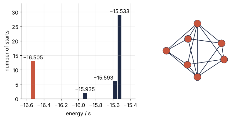
This is the figure from the top. The tallest bar is not the answer. The answer is the leftmost bar, and the only way to know it is leftmost is to have started often enough to see it more than once.

Pitfalls

Trusting fun without reading success. Nelder-Mead in Step 4 returned −14.744 ε, a plausible energy for seven atoms that is no minimum at all: it is wherever the simplex happened to be when the budget ran out, and success False says so. Check res.success in every loop. When it is False, raise the limit through the options dictionary, options={"maxfev": 20000} for Nelder-Mead or options={"maxiter": 2000} for BFGS, or better, give a gradient and use a gradient method. True is no guarantee either: it says only that the method's own stopping test passed, for BFGS the small gradient of Step 2, and the third pitfall shows what that test lets through.

Coordinates in the wrong shape. Pass the positions as a (7, 3) array and minimize stops at once with ValueError: 'x0' must only have one dimension. A gradient that returns shape (7, 3) instead of (21,) breaks the same way. The rule is flat outside, shaped inside: ravel() going in, reshape(-1, 3) inside the function, ravel() on the gradient.

Starting atoms on top of each other, or far apart. Drop the 0.8 σ rule from random_start and run the same fifty minimizations:

def farthest_neighbor(x):
    """The largest distance from any atom to its nearest neighbor."""
    d = squareform(pdist(x.reshape(-1, 3)))
    np.fill_diagonal(d, np.inf)
    return d.min(axis=1).max()

rng_raw = np.random.default_rng(1)
starts = [rng_raw.uniform(0, 2, 21) for _ in range(50)]
raw = [minimize(energy, s, jac=gradient) for s in starts]
E_raw = np.array([r.fun for r in raw])
print(f"{sum(r.success for r in raw)} of 50 report success, {(E_raw > -15.5).sum()} end above -15.5 ε")

lost = np.isclose(E_raw, -12.303, atol=1e-3)
closest = np.array([pdist(s.reshape(-1, 3)).min() for s in starts])[lost]
gone = np.array([farthest_neighbor(r.x) for r in raw])[lost]
print(f"{lost.sum()} end at -12.303 ε; closest pair at the start {closest.min():.2f} to {closest.max():.2f} σ;"
      f" lone atom {gone.min():.0f} to {gone.max():.0f} σ from the rest")

rest = (E_raw > -15.5) & ~lost
print(f"the other {rest.sum()} end at", ", ".join(f"{E + 0.0:.3f}" for E in np.unique(E_raw[rest].round(3))), "ε")

48 of 50 report success, 30 end above -15.5 ε
13 end at -12.303 ε; closest pair at the start 0.30 to 0.53 σ; lone atom 11 to 162 σ from the rest
the other 17 end at -10.106, -9.104, -6.000, -5.160, -3.000, -2.000, -1.000, 0.000 ε

Almost all of them report success, and 30 of the 50 end above −15.5 ε. Step 5 found every seven-atom minimum between −16.505 and −15.533 ε, so none of these 30 is a seven-atom cluster. The 13 at −12.303 ε are a minimum of six atoms plus one atom that left. The other 17 broke up further: −9.104 ε is the five-atom bipyramid of Step 3 with two atoms gone, −3.000 ε the triangle of Step 2, and 0.000 ε seven atoms that ended far from each other. Each start that ended at −12.303 ε had a pair closer than 0.55 σ, where the repulsion is \(10^4\) to \(10^7\) ε.

The first step throws one atom far out, and the attraction it feels there, \(24 r^{-7}\), is below gtol from about 8 σ on. Once the rest has settled, the gradient is small everywhere, and BFGS reports success, exactly as Step 2 said it would. A start box much wider than the cluster does the same without any overlap: an atom that begins more than 8 σ from all the others adds nothing above gtol to the gradient. Keep a minimum distance in the start generator, and check the result by counting neighbors, as in Step 5. For a function that is not atoms in a box the rule is the same: spread the starts over the region where a sensible answer can lie, and keep them out of places where the function blows up.

Variations

Basin hopping. scipy.optimize.basinhopping(energy, x0, minimizer_kwargs={"jac": gradient}) automates the restarts: it kicks the coordinates at random and minimizes again from there, many times. The method comes from the same paper as the reference energies (Wales and Doye, 1997).
Thirteen atoms. Call random_start(13, side=2.5): in the default cube of side 2 σ about one draw in ten million keeps every pair 0.8 σ apart, at 2.5 σ about one in four thousand. The global minimum is the icosahedron at −44.326801 ε. Count the hits on it and the distinct end energies among fifty starts as in Step 5, and compare with the 13 hits and four energies of seven atoms: far fewer hits, far more end energies. Plain restarts stop scaling here.
Bounds. method="L-BFGS-B", bounds=[...] with one (low, high) pair per variable, None for a side without a limit, keeps the search in a box, for example atoms adsorbed on a surface with \(z \ge 0\), which is (0, None) for every \(z\) coordinate.
Fitting. A sum of squared residuals, or a negative log-likelihood for noise that is not Gaussian, is minimized with the same call. For the first, scipy.optimize.curve_fit does the work and adds the uncertainties, as in Fit a curve to data with error bars and draw a confidence band.

Cheat sheet

res = minimize(f, x0,                       # f(x) returns a float; x0 is flat, shape (n,)
               jac=grad,                    # grad(x) returns shape (n,); check it with approx_fprime
               method="BFGS",               # default without bounds; "Nelder-Mead" needs no gradient
               options={"maxiter": 2000})   # "maxfev" for Nelder-Mead
res.x, res.fun                              # where it stopped and the value there
res.success, res.message                    # read both: success means a stopping test passed
res.nfev, res.nit                           # cost meter
minimize(f, x0, jac=grad, method="L-BFGS-B", bounds=[(lo, hi)] * n)       # box constraints
best = min((minimize(f, s, jac=grad) for s in starts), key=lambda r: r.fun)   # restarts