Filtering with scipy.signal: mains hum and noise out of an ECG

The problem: a heartbeat under mains hum

Here is one lead of an electrocardiogram, 10 s at 500 samples per second, with an R wave of 1.2 mV, and it needs filtering. A cheap front end or a loose electrode has added 50 Hz hum from the mains at 0.30 mV, a quarter of the R wave, and broadband noise on top. The raw record is off from the true heartbeat by 0.22 mV RMS, and on screen it is a fuzzy band with spikes in it. You want the heartbeat back, with the R peak at its true height and its true time, and scipy.signal has the filters for it.

The record is synthetic, a sum of five bumps per beat that is a cartoon of a real lead but close enough in shape and spectrum for the filter choices to carry over. It is synthetic so that the answer can be checked against the truth.

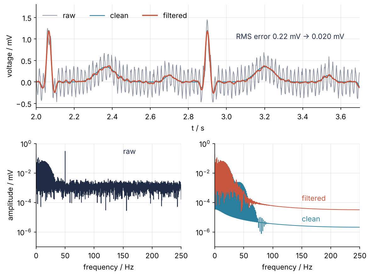
This is where we end up. A notch at 50 Hz and a Butterworth low-pass at 40 Hz, both run forward and backward over the record, bring the RMS error down by a factor of eleven, take the hum line down by a factor of almost 500, and leave the R peak where it was. The spectra are the ones from The Fourier transform: asking a signal how much of each frequency it contains, which mentions removing hum by zeroing the spectrum at 50 Hz. The filters here do that job sample by sample, and Step 2 says why that matters.

Setup

Each beat is five Gaussians, the P, Q, R, S, and T waves, at fixed offsets from the R peak. The clean ecg, the hum, and the noise stay separate arrays so that every part can be filtered on its own later.

import numpy as np
import matplotlib.pyplot as plt
from scipy import signal

fs = 500.0                                   # sampling rate, Hz
t = np.arange(0, 10, 1 / fs)                 # s
rng = np.random.default_rng(42)

# (offset from the R peak / s, amplitude / mV, width / s) for P, Q, R, S, T
waves = [(-0.20, 0.15, 0.025), (-0.03, -0.15, 0.008), (0.0, 1.20, 0.010),
         (0.03, -0.25, 0.008), (0.30, 0.35, 0.050)]
r_times = np.arange(0.4, 10, 60 / 72)        # 72 beats per minute
ecg = np.zeros_like(t)
for t_r in r_times:
    for offset, amp, width in waves:
        ecg += amp * np.exp(-0.5 * ((t - t_r - offset) / width) ** 2)

hum = 0.30 * np.cos(2 * np.pi * 50 * t + 0.7)   # the mains phase at the start is arbitrary
noise = 0.05 * rng.standard_normal(t.size)
x = ecg + hum + noise                        # what the amplifier delivers, mV

def rms(d):
    return np.sqrt(np.mean(d ** 2))

plt.rcParams.update({
    "figure.figsize": (7, 3.6), "figure.dpi": 110,
    "axes.spines.top": False, "axes.spines.right": False,
    "axes.grid": True, "grid.alpha": 0.25,
    "font.size": 11, "lines.linewidth": 1.8,
})
INK, ACCENT, SECOND, MUTED = "#1f2a44", "#c8553d", "#2a7f9e", "#8a8f98"

print(f"{t.size} samples at {fs:.0f} Hz, raw record off by {rms(x - ecg):.2f} mV RMS")

5000 samples at 500 Hz, raw record off by 0.22 mV RMS

Step 1: Look at the spectrum of the raw record

The amplitude spectrum is rfft scaled by 2/N, as in the Fourier tutorial, so a line of amplitude 0.30 mV shows up as 0.30 mV. Plot it on a logarithmic axis: the hum is 250 times the noise floor, and on a linear axis everything but the hum would be flat. From the next step on, gains are in decibels: 20 log10 of an amplitude ratio, so -20 dB is a factor of 10 and -3 dB a factor of 0.71.

Copy

freq = np.fft.rfftfreq(t.size, d=1 / fs)

def amplitude(s):
    return 2 * np.abs(np.fft.rfft(s)) / s.size   # mV

A_raw = amplitude(x)
k50 = np.argmin(np.abs(freq - 50))
floor_raw = np.median(A_raw[freq > 100])
print(f"hum line        {A_raw[k50]:.2f} mV at {freq[k50]:.1f} Hz")
for n in (5, 20, 34):
    f_n = n * 72 / 60                        # the n-th harmonic of the heart rate
    print(f"harmonic {n:2d}     {A_raw[np.argmin(np.abs(freq - f_n))]:.4f} mV at {f_n:.1f} Hz")
print(f"noise floor     {floor_raw:.4f} mV (median above 100 Hz)")

fig, ax = plt.subplots()
ax.semilogy(freq, A_raw, color=INK, lw=1.0)
ax.axvline(40, color=MUTED, ls="--", lw=1)
ax.text(38, 2e-5, "40 Hz", color=MUTED, ha="right")
ax.text(53, 0.2, "hum, 0.30 mV", color=INK)
ax.text(3, 0.18, "ECG\nharmonics", color=INK, va="bottom")
ax.text(150, 0.005, "noise floor", color=INK)
ax.set(xlabel="frequency / Hz", ylabel="amplitude / mV", xlim=(0, 250), ylim=(1e-5, 2))
plt.show()

hum line        0.30 mV at 50.0 Hz
harmonic  5     0.0780 mV at 6.0 Hz
harmonic 20     0.0250 mV at 24.0 Hz
harmonic 34     0.0020 mV at 40.8 Hz
noise floor     0.0012 mV (median above 100 Hz)

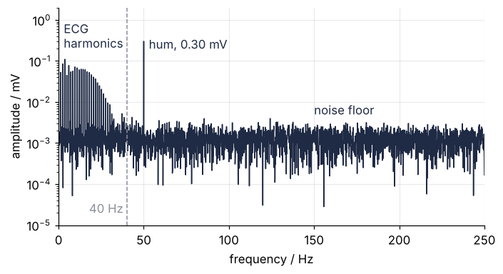
The heartbeat is a comb of lines at multiples of 1.2 Hz, the heart rate. They fall from 0.08 mV at 6 Hz to 0.002 mV at 40 Hz, less than twice the noise floor, and above that only the hum spike stands out of the noise. Two decisions come straight off this picture: cut above about 40 Hz, and take out 50 Hz separately, because it sits too close to 40 Hz for one cut to do both.

Step 2: Design a notch for the hum and read its response

Zeroing the spectrum at 50 Hz and transforming back, the repair the Fourier tutorial mentions, needs the whole record at once. A digital filter works sample by sample instead: each output is a weighted sum of the last few inputs and the last few outputs, so it runs on a record of any length and while the data arrives. The weights are two arrays, b for the inputs and a for the outputs, which a design function returns and the filtering functions take. What the filter does to each frequency is still a factor in the spectrum, and freqz computes that factor, the frequency response, whose magnitude in dB is the gain.

iirnotch designs a notch from its center frequency and its quality factor Q, the center frequency divided by the width of the notch at -3 dB:

Copy

b, a = signal.iirnotch(50, Q=30, fs=fs)

f_check = [45, 49, 50, 51, 55]
_, h = signal.freqz(b, a, worN=f_check, fs=fs)
for f_c, g in zip(f_check, 20 * np.log10(np.abs(h))):
    print(f"{f_c:3d} Hz  {g:8.2f} dB")

w, h = signal.freqz(b, a, worN=8192, fs=fs)
gain = 20 * np.log10(np.abs(h))
stop = w[gain < -3]
print(f"-3 dB band  {stop.min():.1f} to {stop.max():.1f} Hz")

fig, ax = plt.subplots()
ax.plot(w, gain, color=ACCENT)
ax.axhline(-3, color=MUTED, ls="--", lw=1)
ax.text(31, -6.5, "−3 dB", color=MUTED)
ax.text(52, -20, f"below −3 dB\n{stop.min():.1f} to {stop.max():.1f} Hz", color=ACCENT)
ax.set(xlabel="frequency / Hz", ylabel="gain / dB", xlim=(30, 70), ylim=(-40, 3))
plt.show()

 45 Hz     -0.11 dB
 49 Hz     -2.26 dB
 50 Hz   -285.10 dB
 51 Hz     -2.32 dB
 55 Hz     -0.13 dB
-3 dB band  49.2 to 50.8 Hz

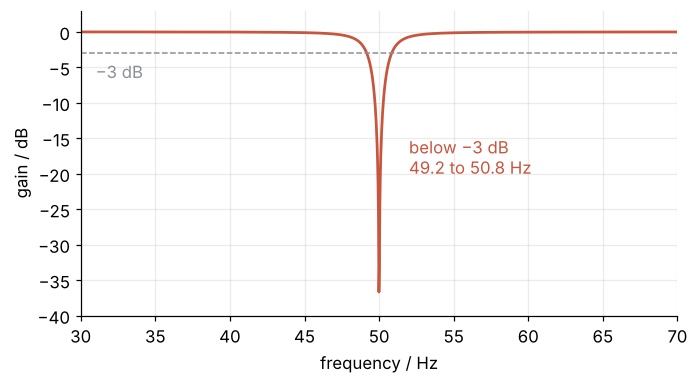
With Q = 30 the notch is 50/30 = 1.7 Hz wide at -3 dB, which the printout, on a grid of 0.03 Hz, finds as 49.2 to 50.8 Hz. Outside 45 to 55 Hz it costs the signal at most 0.13 dB. At exactly 50 Hz the gain is -285 dB, zero to any precision you will meet, so the plot stops at -40 dB. A higher Q would spare more of the signal near 50 Hz but would take longer to settle, a trade that comes back in the third pitfall.

Step 3: Design a Butterworth low-pass and choose its order

A low-pass keeps the band below its cutoff, the passband, and suppresses what lies above. Butterworth is the design whose gain in the passband is as flat as possible, nothing more. The order is the number of past outputs each new output is computed from (its poles, in textbook terms), and each one steepens the fall beyond the cutoff. output="sos" returns the filter as a chain of second-order sections, stages of two poles each, so order 4 is two sections. The SciPy documentation recommends this form for filtering because the single (b, a) pair loses precision as the order grows. Compare three orders at the same 40 Hz cutoff:

Copy

f_check = [20, 30, 40, 50, 100]
print("order" + "".join(f"{f_c:>8d} Hz" for f_c in f_check))

fig, ax = plt.subplots()
for N, alpha in [(2, 0.35), (4, 0.65), (8, 1.0)]:
    sos_N = signal.butter(N, 40, fs=fs, output="sos")
    _, h = signal.freqz_sos(sos_N, worN=f_check, fs=fs)
    print(f"{N:5d}" + "".join(f"{g:8.1f} dB" for g in 20 * np.log10(np.abs(h))))
    w, h = signal.freqz_sos(sos_N, worN=4096, fs=fs)
    gain = 20 * np.log10(np.abs(h))
    k = np.argmin(np.abs(w - 103))                   # label each line just above it at 103 Hz
    ax.plot(w, gain, color=ACCENT, alpha=alpha)
    ax.text(w[k], gain[k] + 2, f"order {N}", color=ACCENT, va="bottom")
ax.axvline(40, color=MUTED, ls="--", lw=1)
ax.axvline(50, color=MUTED, ls="--", lw=1)
ax.text(39, -75, "cutoff", color=MUTED, ha="right")
ax.text(51, -75, "hum", color=MUTED)
ax.set(xlabel="frequency / Hz", ylabel="gain / dB", xlim=(0, 150), ylim=(-80, 3))
plt.show()

sos = signal.butter(4, 40, fs=fs, output="sos")

order      20 Hz      30 Hz      40 Hz      50 Hz     100 Hz
    2    -0.2 dB    -1.2 dB    -3.0 dB    -5.5 dB   -18.1 dB
    4    -0.0 dB    -0.4 dB    -3.0 dB    -8.8 dB   -36.1 dB
    8    -0.0 dB    -0.0 dB    -3.0 dB   -16.5 dB   -72.3 dB

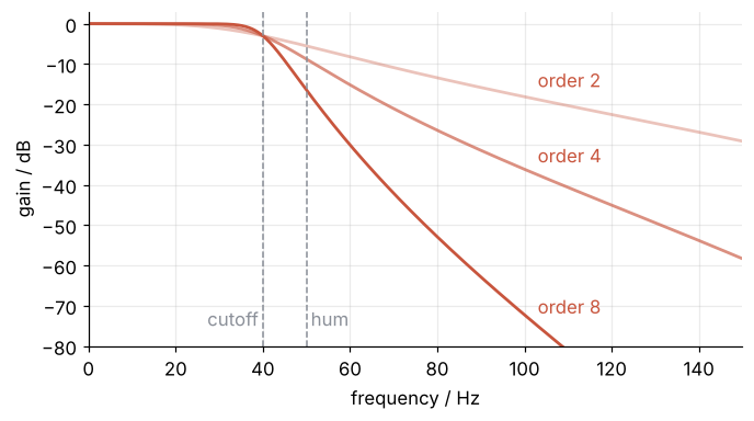
All three are at -3 dB at the cutoff, by design. The order buys steepness in proportion, which the 100 Hz column shows: -18, -36, -72 dB. The textbook rule of 6 dB per octave (a doubling of frequency) per order predicts -32 dB for order 4 at 100 Hz, 1.3 octaves up; this digital filter does a little better because its gain dives to zero at 250 Hz, half the sampling rate. At 50 Hz even order 8 gets only to -16.5 dB, which is why the hum gets its own notch. Order 4 is the choice, and the first pitfall says what a higher order costs.

Step 4: Apply it forward and backward with filtfilt

A filter running on data as it arrives is causal: it can use only the present and past samples. Every causal filter shifts the phase of each frequency as well as scaling its amplitude, which in time means it holds each frequency back by its own delay, the group delay. For an ECG that matters, because the time of the R peak is the measurement.

lfilter(b, a, x) runs the filter once, front to back, as a live filter would. filtfilt(b, a, x) runs it front to back, then back to front over the result. It first extends the record at each end by a few samples, an upside-down mirror image of the end, for the filter to start up on, and cuts them off afterwards. sosfilt and sosfiltfilt do the same with second-order sections, and find_peaks locates the R peaks as maxima above height, at least distance samples apart:

Copy

y_causal = signal.sosfilt(sos, signal.lfilter(b, a, x))
y = signal.sosfiltfilt(sos, signal.filtfilt(b, a, x))

r_true, _ = signal.find_peaks(ecg, height=0.8, distance=200)
shift = {}
for name, out in [("lfilter + sosfilt", y_causal), ("filtfilt + sosfiltfilt", y)]:
    r_out, _ = signal.find_peaks(out, height=0.8, distance=200)
    shift[name] = (r_out - r_true).mean() / fs * 1000
    print(f"{name:23s} R peaks {shift[name]:5.1f} ms late, RMS error {rms(out - ecg):.3f} mV")

beat = (t > 1.80) & (t < 2.45)
fig, axes = plt.subplots(2, 1, sharex=True, figsize=(7, 4.4))
for ax, (name, out) in zip(axes, [("lfilter + sosfilt", y_causal), ("filtfilt + sosfiltfilt", y)]):
    ax.plot(t[beat], ecg[beat], color=SECOND, lw=1.2)
    ax.plot(t[beat], out[beat], color=ACCENT)
    ax.axvline(r_times[2], color=MUTED, ls="--", lw=1)
    ax.text(2.11, 0.9, f"{name}: R peak {shift[name]:.0f} ms late", color=ACCENT)
    ax.set(ylabel="voltage / mV")
axes[0].text(1.82, 0.45, "clean ECG", color=SECOND)
axes[1].set(xlabel="t / s", xlim=(1.80, 2.45))
plt.show()

lfilter + sosfilt       R peaks  11.0 ms late, RMS error 0.144 mV
filtfilt + sosfiltfilt  R peaks   0.0 ms late, RMS error 0.020 mV

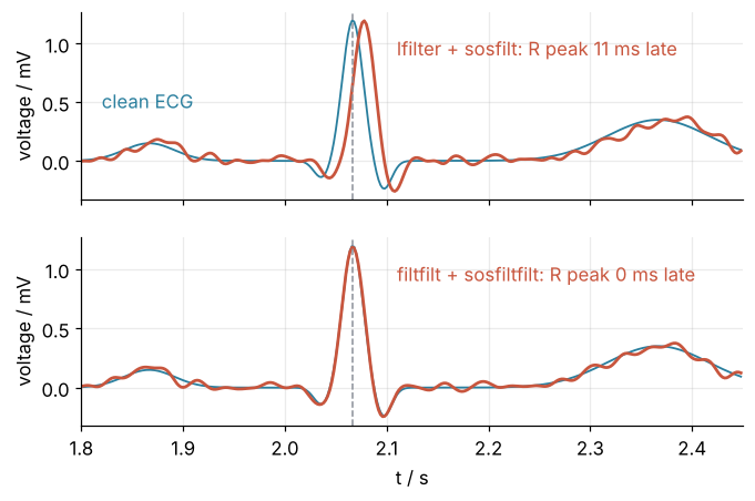
The causal chain puts the R peaks 11 ms late on average, and most of its 0.14 mV error is that delay. Forward and backward gives 0 ms and 0.020 mV: the backward pass shifts every frequency by the same amount the other way, and the two shifts cancel. A filter with no net phase shift is called zero-phase.

The price is that the gain is applied twice, so the low-pass is -6 dB at 40 Hz, not -3. Square the response to find the -3 dB point of the pair, for the design at 40 Hz and for one at 45 Hz:

def f_3dB(sos_f):
    w, h = signal.freqz_sos(sos_f, worN=8192, fs=fs)
    return w[np.argmax(np.abs(h) ** 2 < 10 ** (-3 / 20))]   # gain squared: applied twice
print(f"-3 dB point under sosfiltfilt: designed at 40 Hz {f_3dB(sos):.1f} Hz, "
      f"designed at 45 Hz {f_3dB(signal.butter(4, 45, fs=fs, output='sos')):.1f} Hz")

-3 dB point under sosfiltfilt: designed at 40 Hz 36.0 Hz, designed at 45 Hz 40.5 Hz

The pair is down 3 dB at 36 Hz. If you need -3 dB at 40 Hz under sosfiltfilt, design at 45 Hz. Here 40 Hz stays, because in the Step 1 spectrum nothing between 36 and 40 Hz stands clear of the noise.

Step 5: Check in the spectrum what went and what stayed

Compare the cleaned record with the raw one and the truth:

A_y, A_ecg = amplitude(y), amplitude(ecg)
floor_y = np.median(A_y[freq > 100])
print(f"50 Hz line          {A_raw[k50]:.2f} mV -> {A_y[k50]:.4f} mV")
print(f"floor above 100 Hz  {floor_raw:.4f} mV -> {floor_y:.6f} mV, "
      f"{20 * np.log10(floor_y / floor_raw):.0f} dB")
print(f"RMS error           {rms(x - ecg):.2f} mV -> {rms(y - ecg):.3f} mV")
print(f"R peak height       {100 * np.mean(y[r_true] / ecg[r_true]):.0f} % of the truth")

50 Hz line          0.30 mV -> 0.0006 mV
floor above 100 Hz  0.0012 mV -> 0.000037 mV, -30 dB
RMS error           0.22 mV -> 0.020 mV
R peak height       98 % of the truth

The hum line is down by a factor of almost 500 and the R peaks keep 98 % of their height. The floor above 100 Hz is down by only 30 dB, though the filter gain there is below -72 dB, Step 3's -36 dB at 100 Hz applied twice by sosfiltfilt. The transform treats the record as one period of a repeating signal, so the last sample jumps back to the first. A jump takes every frequency to build, at amplitudes that fall slowly. A ramp with the same jump is smooth everywhere else, so its spectrum is the jump's alone:

jump = y[-1] - y[0]
ramp = jump * t / t[-1]
print(f"jump last to first  {jump:+.3f} mV; ramp floor {np.median(amplitude(ramp)[freq > 100]):.6f} mV")
for name, part in [("hum", hum), ("noise", noise), ("ECG", ecg)]:
    part_out = signal.sosfiltfilt(sos, signal.filtfilt(b, a, part))   # filters are linear: shares add up
    print(f"  from the {name:5s}  {part_out[-1] - part_out[0]:+.3f} mV")

jump last to first  -0.123 mV; ramp floor 0.000028 mV
  from the hum    -0.074 mV
  from the noise  -0.061 mV
  from the ECG    +0.012 mV

The ramp makes three quarters of the floor. Of the jump, 0.07 mV is hum left at the edges (the third pitfall) and 0.06 mV noise.

The error left is 0.020 mV, and you can predict it. White noise spreads its power evenly up to the Nyquist frequency, 250 Hz here, and a filter that keeps 0 to 40 Hz keeps 40/250 of it. RMS is the square root of power, so 0.05 mV times √(40/250) survives:

predicted = 0.05 * np.sqrt(40 / (fs / 2))
noise_left = signal.sosfiltfilt(sos, signal.filtfilt(b, a, noise))
print(f"in-band noise: predicted {predicted:.3f} mV, noise filtered alone {rms(noise_left):.3f} mV")
ecg_left = signal.sosfiltfilt(sos, signal.filtfilt(b, a, ecg))
print(f"ECG filtered alone: off from the truth by {rms(ecg_left - ecg):.3f} mV")

in-band noise: predicted 0.020 mV, noise filtered alone 0.019 mV
ECG filtered alone: off from the truth by 0.004 mV

The two agree to within 5 %; the gap is the cutoff being a slope, not a wall. The heartbeat filtered alone loses 0.004 mV, a fifth of that. What is left is noise inside the heartbeat's band, which no filter removes. For your own record the same square root predicts this error before you filter.

Copy

fig = plt.figure(figsize=(8, 6))
grid = fig.add_gridspec(2, 2, height_ratios=[1, 1])
ax_t = fig.add_subplot(grid[0, :])
two = (t > 2.0) & (t < 3.7)
ax_t.plot(t[two], x[two], color=INK, lw=1.0, alpha=0.5, label="raw")
ax_t.plot(t[two], ecg[two], color=SECOND, lw=1.2, label="clean")
ax_t.plot(t[two], y[two], color=ACCENT, label="filtered")
ax_t.text(3.05, 1.0, f"RMS error {rms(x - ecg):.2f} mV → {rms(y - ecg):.3f} mV", color=INK)
ax_t.set(xlabel="t / s", ylabel="voltage / mV", xlim=(2.0, 3.7), ylim=(-0.6, 1.8))
ax_t.legend(frameon=False, loc="upper left", ncols=3)

ax_b = fig.add_subplot(grid[1, 0])
ax_a = fig.add_subplot(grid[1, 1], sharey=ax_b)
ax_b.semilogy(freq, A_raw, color=INK, lw=1.0)
ax_b.text(150, 0.2, "raw", color=INK)
ax_a.semilogy(freq, A_ecg, color=SECOND, lw=1.0)
ax_a.semilogy(freq, A_y, color=ACCENT, lw=1.0)
ax_a.text(150, 1e-4, "filtered", color=ACCENT, va="bottom")
ax_a.text(150, 4e-6, "clean", color=SECOND, va="bottom")
for ax in (ax_b, ax_a):
    ax.set(xlabel="frequency / Hz", xlim=(0, 250), ylim=(1e-7, 1))
ax_b.set(ylabel="amplitude / mV")
fig.tight_layout()
plt.show()

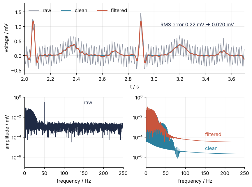
Below 40 Hz the filtered spectrum lies on the clean ECG's. Above, it drops away, taking the clean ECG's 0.002 mV lines between 40 and 55 Hz, the 0.004 mV the heartbeat lost. Above about 90 Hz it is smooth, the spectrum of that one jump.

Pitfalls

Turning up the order until it rings. The symptom is ripples on both sides of every sharp edge, a fake wiggle before and after the QRS complex. A filter with a steep cutoff answers a single sharp spike with a long decaying wiggle (its impulse response), and every sharp edge in the signal sets that wiggle off. The steeper the cutoff, the larger the wiggle. Feed a unit step through the zero-phase low-pass:

step = np.r_[np.zeros(500), np.ones(500)]
for N in (2, 4, 8):
    s = signal.sosfiltfilt(signal.butter(N, 40, fs=fs, output="sos"), step)
    print(f"order {N}: overshoot {100 * (s.max() - 1):.1f} %, undershoot {100 * -s[:500].min():.1f} %")

order 2: overshoot 3.6 %, undershoot 3.6 %
order 4: overshoot 6.9 %, undershoot 6.9 %
order 8: overshoot 8.4 %, undershoot 8.4 %

The zero-phase filter rings before the edge as well as after it, by the same amount: 3.6 % at order 2, 6.9 % at order 4, 8.4 % at order 8. Use the lowest order that does the job, read off the response in Step 3.

Forgetting fs and the normalized frequency. butter(4, 40) raises an error, and the common repair butter(4, 40 / fs) silently gives the wrong cutoff. Without fs, SciPy measures frequency in units of the Nyquist frequency fs / 2, not of fs, so 40 / 500 means 20 Hz:

try:
    signal.butter(4, 40)
except ValueError as err:
    print("ValueError:", err)
w, h = signal.freqz_sos(signal.butter(4, 40 / fs, output="sos"), worN=8192, fs=fs)
print(f"butter(4, 40 / fs) is -3 dB at {w[np.argmax(np.abs(h) < 10 ** (-3 / 20))]:.1f} Hz")

ValueError: Digital filter critical frequencies must be 0 < Wn < 1
butter(4, 40 / fs) is -3 dB at 20.0 Hz

Half the cutoff you asked for, and nothing in the output warns you. Always pass fs=fs to the design and to freqz; every frequency is then in hertz.

Trusting the first and last half second. Hum survives at the start and end of the record, while the middle is clean. Filter the hum alone and look at the edges:

hum_left = signal.filtfilt(b, a, hum)
n01, n05 = int(0.1 * fs), int(0.5 * fs)
print(f"first 0.1 s            {np.abs(hum_left[:n01]).max():.3f} mV")
print(f"same, method=\"gust\"    {np.abs(signal.filtfilt(b, a, hum, method='gust')[:n01]).max():.3f} mV")
print(f"0.5 s from either end  {np.abs(hum_left[n05:-n05]).max():.3f} mV")
print(f"between 4 and 6 s      {np.abs(hum_left[(t > 4) & (t < 6)]).max():.0e} mV")

first 0.1 s            0.147 mV
same, method="gust"    0.287 mV
0.5 s from either end  0.011 mV
between 4 and 6 s      1e-10 mV

Half the hum is still there in the first 0.1 s, and a billion times less in the middle. A narrow notch has to see many cycles of the hum before it cancels it, about Q/(π f0) = 0.19 s here, the slow settling that Step 2 traded for a narrow notch. The extension that filtfilt adds at each end is 9 samples for the notch, 18 ms, and an upside-down mirror image of the hum is not the hum. A longer padlen or another padtype ("even", "constant") helps for some phases of the mains and not for others. method="gust", which drops the extension and chooses the start values of both passes instead, leaves more hum at every phase. Record a little longer than you need and discard about 0.5 s at each end, which leaves 0.011 mV, or lower Q if the edges matter.

Variations

• Baseline wander. Breathing and electrode motion add drift below 0.5 Hz. Replace the low-pass with signal.butter(2, [0.5, 40], btype="bandpass", fs=fs, output="sos").
• 60 Hz and its harmonics. In North America the mains is 60 Hz, and nonlinear loads on the supply add lines at 120 and 180 Hz. signal.iircomb(60, Q=30, fs=fs) notches the whole series, but only when fs is a whole multiple of 60, so sample at 600 Hz or chain one iirnotch per harmonic.
• Filtering as the data arrives. A monitor cannot look into the future. Use sosfilt with the initial state from signal.sosfilt_zi, carry the state zi from chunk to chunk, and accept the 11 ms delay from Step 4.
• A strain gauge instead of a heart. A bridge sampled at 1 kHz with a load signal below 20 Hz takes the same chain; only fs, the cutoff, and the notch frequency change.

Cheat sheet

b, a = signal.iirnotch(f0, Q, fs=fs)                  # notch; -3 dB width f0 / Q
sos = signal.butter(N, fc, btype="low", fs=fs, output="sos")   # always fs=, always sos
w, h = signal.freqz(b, a, fs=fs)                      # response of (b, a); gain 20*log10(|h|)
w, h = signal.freqz_sos(sos, fs=fs)                   # response of sos
y = signal.sosfiltfilt(sos, signal.filtfilt(b, a, x)) # zero phase; gain applied twice, -6 dB at fc
y = signal.sosfilt(sos, signal.lfilter(b, a, x))      # causal; delayed by the group delay
zi = signal.sosfilt_zi(sos) * x[0]                    # start state for chunked sosfilt(..., zi=zi)
sigma * np.sqrt(fc / (fs / 2))                        # white noise left in the band 0 to fc
y = y[int(0.5 * fs):-int(0.5 * fs)]                   # drop edges, a few notch settling times Q/(pi f0)

Further reading

• The SciPy reference for butter, iirnotch, filtfilt, and sosfiltfilt, and the overview of scipy.signal.
• Steven W. Smith, The Scientist and Engineer's Guide to Digital Signal Processing, for the filter chapters, and Oppenheim and Schafer, Discrete-Time Signal Processing, for the theory behind them.
• Related tutorials on this site: The Fourier transform: asking a signal how much of each frequency it contains. Planned: The same filters in Julia with DSP.jl and Spectral analysis with scipy.signal: windows, leakage, and the periodogram.
• Download the notebook. It was executed with the library versions in the header.