scipy.stats from the ground up: is the difference between two samples real?

Afterwards you can describe two samples with scipy.stats, test whether they differ, and report the effect size with a confidence interval, not a bare p-value.

Topic: Statistics
Field: Cross-disciplinary
Libraries: matplotlib 3.11.2, numpy 2.5.3, scipy 1.18.1
Prerequisites: none beyond Python basics
Notebook: Download py-scipy-stats-two-samples.ipynb, executed with the versions above

The problem: is a 4.6 % higher yield real?

A preparation is run in twelve batches with the standard protocol A and in twelve with a modified protocol B, and the product of every batch is weighed. The B batches come out at 51.68 mg on average, 2.26 mg or 4.6 % more than the A batches. But the batches of either protocol scatter by about 2.4 mg, more than the gain. Is the gain real, or is it what twelve noisy numbers do on their own? scipy.stats has the tools to answer that. A chemist reads the example as a synthesis yield, a biologist as protein harvested from a culture; from here on it is just the yield.

With scipy.stats you describe both samples, put an interval on each mean, test the difference, report its size with an interval, and simulate what chance alone produces. The data are simulated, so the true answer is known, and the last step checks every verdict against it.

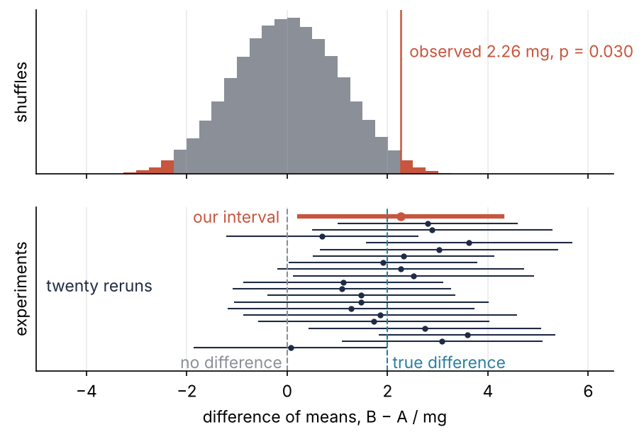
Top: histogram of the difference of means B − A over 100,000 random relabelings of the 24 yields, with the tails beyond the observed 2.26 mg shaded. Bottom: the 95 % confidence interval of the observed difference and of twenty simulated repeats of the experiment, against dashed lines at the true difference of 2 mg and at zero.

This is where we end up. The top panel is what chance produces when the labels A and B are shuffled, with the observed difference out in the tail; the bottom panel puts our interval for the difference among those of twenty reruns of the same experiment. Shuffles are Step 5 and reruns are Step 6. The verdict it previews: chance rarely produces a gain this large, and the true gain lies anywhere from 0.5 % to 8.7 %.

Setup

Everything below draws from one seeded generator:

import numpy as np
import matplotlib.pyplot as plt
from scipy import stats

# the truth, which a real experiment never shows you; used again only in Step 6
mu_A, mu_B = 50.0, 52.0     # true mean yields, mg
sigma = 2.5                 # true batch-to-batch scatter, mg
n = 12                      # batches per protocol

rng = np.random.default_rng(159)
a = np.round(rng.normal(mu_A, sigma, n), 1)     # a balance records 0.1 mg
b = np.round(rng.normal(mu_B, sigma, n), 1)

plt.rcParams.update({
    "figure.figsize": (7, 3.6), "figure.dpi": 110,
    "axes.spines.top": False, "axes.spines.right": False,
    "axes.grid": True, "grid.alpha": 0.25,
    "font.size": 11, "lines.linewidth": 1.8,
})
INK, ACCENT, SECOND, MUTED = "#1f2a44", "#c8553d", "#2a7f9e", "#8a8f98"

print("A:", a)
print("B:", b)

A: [48.3 47.  51.9 49.3 52.5 50.3 48.7 50.5 52.5 47.1 49.7 45.3]
B: [50.9 50.9 49.1 55.5 55.1 51.8 51.7 52.9 49.1 55.  49.9 48.3]

Step 1: Describe each sample with stats.describe

stats.describe(x) returns the count, the minimum and maximum, the mean, the variance, the skewness, and the kurtosis in one call. Printed raw it is a wall of np.float64(...), so pick the fields and format them:

for name, x in [("A", a), ("B", b)]:
    d = stats.describe(x)
    print(f"{name}: mean {d.mean:5.2f} mg   variance {d.variance:4.2f} mg²   sd {np.sqrt(d.variance):4.2f} mg   "
          f"sem {stats.sem(x):4.2f} mg   skewness {d.skewness:5.2f}")
print(f"a.std() = {a.std():.2f} mg   a.std(ddof=1) = {a.std(ddof=1):.2f} mg")

A: mean 49.43 mg   variance 5.19 mg²   sd 2.28 mg   sem 0.66 mg   skewness -0.19
B: mean 51.68 mg   variance 6.18 mg²   sd 2.49 mg   sem 0.72 mg   skewness  0.33
a.std() = 2.18 mg   a.std(ddof=1) = 2.28 mg

The variance is the average squared distance from the mean, computed with n − 1 in the denominator, and the standard deviation (sd) is its square root, back in mg. The standard error of the mean (sem) is the standard deviation over √n, 0.66 mg for A against an sd of 2.28 mg: it is the scatter of the mean itself, not of the batches. Skewness is zero for a symmetric sample, so −0.19 and 0.33 read as "no long tail"; Pitfall 2 says how far from zero is far at twelve values. The kurtosis measures tail weight, and at twelve values you can ignore it.

The last line is a trap. ddof is the number subtracted from n in the denominator. NumPy's default is 0, so a.std() divides by n, while describe and sem divide by n − 1, and the two answers differ by 4 %. For a sample, which is everything you ever measure, use n − 1.

Step 2: Ask the t distribution for a confidence interval

Within what range around 49.43 mg does the true mean of A plausibly lie? For normally scattered data, the miss of the sample mean in units of its standard error, (mean − true mean) / sem, follows a t distribution with n − 1 = 11 degrees of freedom, the number of values left to estimate the spread once the mean is fixed. The 95 % interval is therefore mean ± c × sem, where c is the multiple the t distribution exceeds in only 2.5 % of experiments in each direction, 5 % in total. That is why the code below asks for 0.975: c is the value with 97.5 % of the distribution below it.

stats.t(df=11) is a distribution object, and three of its methods matter here. cdf(x) is the cumulative probability, the probability of a value at most x. ppf(q) is its inverse, the quantile: the value below which a fraction q lies. sf(x) is 1 − cdf(x), the tail area beyond x.

t11 = stats.t(df=11)
c = t11.ppf(0.975)
print(f"ppf(0.975) = {c:.3f}   cdf({c:.3f}) = {t11.cdf(c):.3f}   sf({c:.3f}) = {t11.sf(c):.3f}")
print(f"normal distribution for comparison: ppf(0.975) = {stats.norm.ppf(0.975):.3f}")

ppf(0.975) = 2.201   cdf(2.201) = 0.975   sf(2.201) = 0.025
normal distribution for comparison: ppf(0.975) = 1.960

The same cut, read three ways. The t value of 2.201 is wider than the normal distribution's 1.960 because the sem is itself estimated from the same twelve values.

Now the interval, by hand and from stats.t.interval, which shifts the t distribution to the mean (loc) and stretches it by the sem (scale):

half_A = c * stats.sem(a)
print(f"A by hand:    {a.mean():.2f} ± {half_A:.2f} = {a.mean() - half_A:.2f} to {a.mean() + half_A:.2f} mg")
for name, x in [("A", a), ("B", b)]:
    low, high = stats.t.interval(0.95, df=n - 1, loc=x.mean(), scale=stats.sem(x))
    print(f"{name} t.interval: {x.mean():.2f} ± {(high - low) / 2:.2f} = {low:.2f} to {high:.2f} mg")

A by hand:    49.43 ± 1.45 = 47.98 to 50.87 mg
A t.interval: 49.43 ± 1.45 = 47.98 to 50.87 mg
B t.interval: 51.68 ± 1.58 = 50.10 to 53.26 mg

This is the confidence interval, and its 95 % is a property of the procedure: an interval built this way catches the true mean in 95 % of experiments. It is not a 95 % probability for this one interval, which either contains the true mean or does not. Step 6 checks the claim.

fig, ax = plt.subplots(figsize=(5, 3.6))
offsets = np.linspace(-0.12, 0.12, n)           # fixed spread in batch order, so no dot hides another
bounds = []
for k, x in enumerate([a, b]):
    ax.plot(k + offsets, x, "o", color=INK, ms=4)
    low, high = stats.t.interval(0.95, df=n - 1, loc=x.mean(), scale=stats.sem(x))
    bounds.append((low, high))
    ax.errorbar(k + 0.3, x.mean(), yerr=[[x.mean() - low], [high - x.mean()]],
                fmt="o", color=ACCENT, ms=6, capsize=3)
ax.fill_between([0.3, 1.3], bounds[1][0], bounds[0][1], color=MUTED, alpha=0.3, lw=0)  # where the intervals overlap
ax.grid(axis="x", visible=False)
ax.set(xticks=[0, 1], xticklabels=["standard (A)", "modified (B)"], xlim=(-0.4, 1.6),
       ylabel="yield / mg")
plt.show()

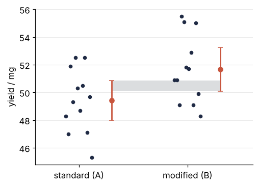
Dots are batches, red bars the means with their 95 % intervals. The batches overlap almost completely, and so do the two intervals, between 50.10 and 50.87 mg. Step 4 shows whether that overlap means the difference could be zero.

Step 3: Test the difference with ttest_ind

stats.ttest_ind compares the means of two independent samples. Put B first: the argument order is the sign of everything that follows, and with B first the difference is B − A and positive. The test divides the difference of the means by its standard error,

\[t = \frac{\bar b - \bar a}{\sqrt{s_a^2/n_a + s_b^2/n_b}} ,\]

with \(\bar a, \bar b\) the sample means, \(s_a, s_b\) the standard deviations, and \(n_a, n_b\) the numbers of batches. The denominator is the standard error of the difference, \(\sqrt{\mathrm{sem}_A^2 + \mathrm{sem}_B^2}\).

res = stats.ttest_ind(b, a, equal_var=False)
diff = b.mean() - a.mean()
se_diff = np.sqrt(stats.sem(a)**2 + stats.sem(b)**2)
print(f"difference {diff:.3f} mg   standard error of the difference {se_diff:.3f} mg")
print(f"t = {res.statistic:.2f}   df = {res.df:.1f}   p = {res.pvalue:.4f}")

difference 2.258 mg   standard error of the difference 0.973 mg
t = 2.32   df = 21.8   p = 0.0301

So t = 2.258 / 0.973 = 2.32. Welch's test, which equal_var=False selects, combines the degrees of freedom of the two samples into one effective number that lies between 11 (one sample) and 22 (both pooled); here it is 21.8. The p-value is the probability of a difference at least this large, in either direction, if the protocol had no effect. That assumption of no effect is the null hypothesis, and p is computed under it. It is not the probability that the null hypothesis is true. Step 2's tail area reproduces it, and equal_var=True runs Student's test, which assumes equal spreads:

p_by_hand = 2 * stats.t.sf(abs(res.statistic), res.df)
student = stats.ttest_ind(b, a, equal_var=True)
print(f"2 × sf(|t|) = {p_by_hand:.4f}")
print(f"Student's test: t = {student.statistic:.2f}   df = {student.df:.0f}   p = {student.pvalue:.4f}")

2 × sf(|t|) = 0.0301
Student's test: t = 2.32   df = 22   p = 0.0300

The two tails beyond ±2.32 hold 3.0 % of the distribution. A test is a statistic plus a tail area, nothing more. Welch's version does not assume that the two spreads are equal and costs little when they are: Student's test gives the same t for equal group sizes and differs only in its 22 degrees of freedom, p = 0.0300 against Welch's 0.0301. Make Welch's your default.

Step 4: Report the size of the difference

The effect size is the size of the difference in the unit you measured, here 2.26 mg. res.confidence_interval() gives its interval, built like Step 2's from the pieces of Step 3: the difference ± c × the standard error of the difference, with c now taken from the t distribution with 21.8 degrees of freedom.

c_diff = stats.t.ppf(0.975, res.df)
half_diff = c_diff * se_diff
ci = res.confidence_interval(confidence_level=0.95)
print(f"c = {c_diff:.3f}   by hand: {diff:.2f} ± {half_diff:.2f} = {diff - half_diff:.2f} to {diff + half_diff:.2f} mg")
print(f"res.confidence_interval(): {ci.low:.2f} to {ci.high:.2f} mg")

c = 2.075   by hand: 2.26 ± 2.02 = 0.24 to 4.28 mg
res.confidence_interval(): 0.24 to 4.28 mg

The interval excludes zero exactly when p < 0.05, because both ask whether |t| = 2.32 exceeds the same cut, 2.075. Now Step 2's question about the overlap. Add the half-widths of A's and B's intervals, and add their standard errors once directly and once in squares:

half_B = c * stats.sem(b)
print(f"half-widths of A and B added: {half_A:.2f} + {half_B:.2f} = {half_A + half_B:.2f} mg")
sem_A, sem_B = stats.sem(a), stats.sem(b)
print(f"standard errors: added {sem_A:.3f} + {sem_B:.3f} = {sem_A + sem_B:.3f} mg, "
      f"in squares √({sem_A:.3f}² + {sem_B:.3f}²) = {se_diff:.3f} mg")

half-widths of A and B added: 1.45 + 1.58 = 3.03 mg
standard errors: added 0.658 + 0.717 = 1.375 mg, in squares √(0.658² + 0.717²) = 0.973 mg

The difference, 2.26 mg, is larger than the half-width of its own interval, 2.02 mg, so that interval excludes zero. It is smaller than the half-widths of A and B together, 3.03 mg, so their intervals overlap. Both hold at once because standard errors add in squares, to 0.973 mg rather than 1.375 mg. Never read overlapping intervals as "no difference".

The report line, with the percentages taken as the bounds divided by A's observed mean:

pct = 100 / a.mean()
print(f"B − A = {diff:.2f} mg ({diff * pct:.1f} % of A), "
      f"95 % CI {ci.low:.2f} to {ci.high:.2f} mg ({ci.low * pct:.1f} % to {ci.high * pct:.1f} %), "
      f"Welch p = {res.pvalue:.3f}")

B − A = 2.26 mg (4.6 % of A), 95 % CI 0.24 to 4.28 mg (0.5 % to 8.7 %), Welch p = 0.030

The lower bound, half a percent, would not justify changing a protocol; the upper, almost 9 %, would. That range is the result, and the p-value only says that it does not reach zero. Fitted parameters get intervals on the same pattern, estimate ± a multiple of its standard error, in Fit a curve to data with error bars and draw a confidence band. There the uncertainties are known in advance, so the multiple is the normal distribution's, about 2 for 95 %, instead of the t distribution's.

Step 5: Simulate the null by shuffling the labels

The argument needs no formula. If the protocol does nothing, the labels A and B are arbitrary, and any split of the 24 yields into two groups of twelve is as likely as the one observed. There are 2,704,156 such splits. stats.permutation_test draws 100,000 of them at random and evaluates your statistic on each. The statistic here is the difference of means, written with an axis argument so that SciPy can evaluate all shuffles in one array call (vectorized=True):

def mean_difference(x, y, axis):
    return np.mean(x, axis=axis) - np.mean(y, axis=axis)

perm = stats.permutation_test((b, a), mean_difference, n_resamples=100_000,
                              vectorized=True, rng=rng)
null = perm.null_distribution
above, below = np.mean(null >= diff), np.mean(null <= -diff)
print(f"null distribution: sd {null.std():.2f} mg")
print(f"shuffles with B − A ≥ +{diff:.2f} mg: {100 * above:.2f} %   ≤ −{diff:.2f} mg: {100 * below:.2f} %")
print(f"permutation p = {perm.pvalue:.4f}")

null distribution: sd 1.06 mg
shuffles with B − A ≥ +2.26 mg: 1.49 %   ≤ −2.26 mg: 1.54 %
permutation p = 0.0298

These 100,000 differences are the null distribution, the differences chance alone produces; its histogram is the top panel of the final figure. They scatter by 1.06 mg, and 3.0 % of them are at least 2.26 mg in either direction, 1.49 % above and 1.54 % below. SciPy's p of 0.0298 doubles the smaller tail, 2 × 1.49 %, instead of adding both, 1.49 % + 1.54 % = 3.03 %. The formula of Step 3 and a brute-force count agree, 0.0301 against 0.0298. That is what makes the formula believable.

Step 6: Check the verdict against the truth

The constants from the setup come back. The true difference is 2.0 mg, and Step 4's interval contains it:

true_diff = mu_B - mu_A
print(ci.low <= true_diff <= ci.high)

True

One experiment says little about the procedure, though. Rerun it 10,000 times with the same truth, all at once, one experiment per row:

def rerun(n, R=10_000):
    """R new experiments with n batches per protocol, drawn from the true constants."""
    A = rng.normal(mu_A, sigma, (R, n))
    B = rng.normal(mu_B, sigma, (R, n))
    return A, B, stats.ttest_ind(B, A, axis=1, equal_var=False)

A, B, rep = rerun(n)
lo, hi = rep.confidence_interval()
covers = (lo <= true_diff) & (true_diff <= hi)
print(f"runs with p < 0.05:          {100 * np.mean(rep.pvalue < 0.05):.1f} %")
print(f"intervals containing 2.0 mg: {100 * np.mean(covers):.1f} %")
print(f"first 20 runs: {covers[:20].sum()} contain 2.0 mg, {(lo[:20] > 0).sum()} lie entirely above zero")

runs with p < 0.05:          45.0 %
intervals containing 2.0 mg: 95.1 %
first 20 runs: 19 contain 2.0 mg, 10 lie entirely above zero

95.1 % of the intervals contain the true difference: that is Step 2's definition of a 95 % interval, checked. Only 45.0 % of the runs reach p < 0.05. That fraction is the power, the chance that an experiment of this size detects a difference that is really there, and at twelve batches it is worse than a coin toss. I picked the seed of this tutorial so that its experiment is one of the 45 %.

fig, (top, bottom) = plt.subplots(2, 1, figsize=(7, 4.4), sharex=True)

# top: the null distribution, with bin edges on ±2.26 mg so that the tails shade cleanly
w = diff / 9
edges = w * np.arange(-21, 27)
counts, _ = np.histogram(null, edges)
centers = edges[:-1] + w / 2
top.bar(centers, counts, width=w, lw=0,
        color=[ACCENT if abs(x) > diff else MUTED for x in centers])
top.axvline(diff, color=ACCENT, lw=1.2)
top.annotate(f"observed {diff:.2f} mg, p = {res.pvalue:.3f}", (diff, 0.75 * counts.max()),
             xytext=(6, 0), textcoords="offset points", color=ACCENT)
top.set(ylabel="shuffles", yticks=[])

# bottom: our interval on top, then the first twenty reruns
rows = np.arange(1, 21)
bottom.plot([ci.low, ci.high], [0, 0], color=ACCENT, lw=3)
bottom.plot(diff, 0, "o", color=ACCENT, ms=5)
bottom.hlines(rows, lo[:20], hi[:20], color=INK, lw=1)
bottom.plot(B[:20].mean(axis=1) - A[:20].mean(axis=1), rows, "o", color=INK, ms=3)
bottom.axvline(true_diff, color=SECOND, lw=1, ls="--")
bottom.axvline(0, color=MUTED, lw=1, ls="--")
bottom.text(true_diff + 0.1, 22.2, "true difference", color=SECOND, va="center")
bottom.text(-0.1, 22.2, "no difference", color=MUTED, ha="right", va="center")
bottom.text(-0.15, 0, "our interval", color=ACCENT, ha="right", va="center")
bottom.text(-4.8, 10.5, "twenty reruns", color=INK, va="center")
bottom.set(xlabel="difference of means, B − A / mg", ylabel="experiments", yticks=[],
           xlim=(-5, 6.5), ylim=(23.5, -1.5))
plt.show()

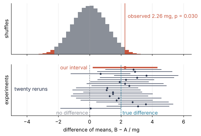
In the first twenty reruns, 19 intervals contain the true 2.0 mg and only ten lie entirely above zero. The other ten are the same experiment, run just as carefully, with an interval that includes zero.

Pitfalls

Trusting p < 0.05 from twelve values. Repeat the experiment and p jumps. Step 6's reruns show how far, and how the runs that reach p < 0.05, the ones usually called significant, compare with all of them:

diffs = B.mean(axis=1) - A.mean(axis=1)
significant = rep.pvalue < 0.05
p10, p90 = np.quantile(rep.pvalue, [0.1, 0.9])
print(f"p over 10,000 reruns: 10th percentile {p10:.3f}, 90th percentile {p90:.3f}")
print(f"mean B − A: all runs {diffs.mean():.2f} mg, runs with p < 0.05 {diffs[significant].mean():.2f} mg")
print(f"26 batches per protocol: p < 0.05 in {100 * np.mean(rerun(26)[2].pvalue < 0.05):.1f} % of runs")

p over 10,000 reruns: 10th percentile 0.003, 90th percentile 0.496
mean B − A: all runs 1.98 mg, runs with p < 0.05 2.84 mg
26 batches per protocol: p < 0.05 in 81.0 % of runs

The same protocols and the same truth give p from 0.003 to 0.496 between the 10th and the 90th percentile. Twelve batches detect a true 4 % gain less than half the time, and the runs that do reach p < 0.05 overestimate it: 2.84 mg on average, against the true 2.0 mg and the 1.98 mg of all runs.

The fix is to report the interval and to treat a single p = 0.03 from twelve batches as a reason to repeat, not as a result. Choose the number of batches before measuring: assign your guesses for the means and the spread to mu_A, mu_B, and sigma, which rerun reads, then call it with growing n until the fraction with p < 0.05 is one you can live with. For this gain, 26 batches per protocol reach 81.0 %.

The t-test on skewed data. Positive quantities that spread by factors, such as concentrations or grain sizes, have a long right tail, and describe shows a skewness well above zero. The cell measures the skewness that chance alone gives normal samples of twelve, on Step 6's reruns, then draws 10,000 pairs of twelve log-normal concentrations (their logarithms are normally scattered), B's median twice A's, and counts how often three tests find the doubling:

s_low, s_high = np.quantile(stats.skew(A, axis=1), [0.025, 0.975])
R = 10_000
a_ln = rng.lognormal(np.log(10), 1.0, (R, n))     # concentrations, µg/L, median 10
b_ln = rng.lognormal(np.log(20), 1.0, (R, n))     # median 20: B is twice A
skew_ln = stats.skew(a_ln, axis=1)
print(f"normal samples: 95 % of skewnesses between {s_low:.2f} and {s_high:.2f}")
print(f"log-normal samples: median skewness {np.median(skew_ln):.2f}, "
      f"{100 * np.mean(skew_ln > s_high):.0f} % above {s_high:.2f}")

found = {
    "t-test on the values": stats.ttest_ind(b_ln, a_ln, axis=1, equal_var=False).pvalue,
    "t-test on the logarithms": stats.ttest_ind(np.log(b_ln), np.log(a_ln), axis=1, equal_var=False).pvalue,
    "mannwhitneyu": stats.mannwhitneyu(b_ln, a_ln, axis=1).pvalue,
}
for name, p in found.items():
    print(f"{name:25s} finds the doubling in {100 * np.mean(p < 0.05):.0f} % of pairs")

normal samples: 95 % of skewnesses between -1.10 and 1.11
log-normal samples: median skewness 1.35, 63 % above 1.11
t-test on the values      finds the doubling in 22 % of pairs
t-test on the logarithms  finds the doubling in 36 % of pairs
mannwhitneyu              finds the doubling in 34 % of pairs

Normal samples of twelve give skewnesses from −1.10 to 1.11 in 95 % of cases, so A's −0.19 and B's 0.33 are ordinary. The log-normal samples have a median skewness of 1.35, yet only 63 % of them exceed 1.11: at twelve values skewness is a hint, and knowing that your quantity spreads by factors is the better guide.

The t-test compares means, which the largest values pull around, so on the raw values it finds the doubling in only 22 % of pairs. On the logarithms, where a ratio becomes a difference, it finds 36 %, and mannwhitneyu, which compares ranks (positions in the sorted pooled sample) rather than means, finds 34 %. Both still miss about two pairs in three, the first pitfall again. Use the logarithms: they find the doubling as often as the ranks do, and they give an effect size with an interval. Exponentiate the difference of the log means and both bounds of its interval, here for the first pair as drawn:

log_res = stats.ttest_ind(np.log(b_ln[0]), np.log(a_ln[0]), equal_var=False)
ratio = np.exp(np.log(b_ln[0]).mean() - np.log(a_ln[0]).mean())
r_low, r_high = np.exp(log_res.confidence_interval())
print(f"B / A = {ratio:.2f}, 95 % CI {r_low:.2f} to {r_high:.2f}, p = {log_res.pvalue:.3f}")

B / A = 1.81, 95 % CI 0.79 to 4.13, p = 0.151

That is the ratio of geometric means (the mean of the logarithms, exponentiated), read as "B is typically 1.8 times A, somewhere between 0.8 and 4.1 times". With p = 0.151 this pair is one of the misses.

Reporting significance without an effect size. "The modified protocol increased the yield significantly (p = 0.03)" does not say by how much. The p-value mixes the size of the difference with the number of batches, and with enough batches any difference, however small, reaches p < 0.05. Report Step 4's line instead.

Variations

Paired measurements. The same specimens are measured before and after a treatment, so the two samples are not independent: use stats.ttest_rel(after, before), which tests the mean of the differences.
Three or more protocols. stats.f_oneway(a, b, c) tests whether any mean differs, and stats.tukey_hsd(a, b, c) then says which pairs do, with intervals.
A standardized effect size. Cohen's d divides the difference by the pooled standard deviation, which for equal group sizes is the square root of the average of the two variances. Write it as cohens_d(x, y, axis) in the shape of Step 5's mean_difference and pass it to stats.bootstrap((b, a), cohens_d) for an interval. With twelve values per group that interval is rough.
Counts instead of measurements. For failed batches out of all batches per protocol, use stats.fisher_exact on the 2 × 2 table.

Cheat sheet

d = stats.describe(x)                          # nobs, minmax, mean, variance (ddof=1), skewness, kurtosis
stats.sem(x), stats.t.interval(0.95, df=len(x) - 1, loc=x.mean(), scale=stats.sem(x))
res = stats.ttest_ind(b, a, equal_var=False)   # Welch; the difference is b − a
res.statistic, res.df, res.pvalue              # t, effective degrees of freedom, two-sided p
res.confidence_interval(0.95)                  # interval of b − a: report this, not p alone
stats.permutation_test((b, a), lambda x, y, axis: x.mean(axis) - y.mean(axis),
                       vectorized=True, n_resamples=100_000)
np.exp(stats.ttest_ind(np.log(b), np.log(a), equal_var=False).confidence_interval())  # skewed: ratio b / a
stats.mannwhitneyu(b, a)                       # compares ranks, not means