Smoothing splines with scipy.interpolate: acceleration from noisy positions

The problem: g from a falling ball's video track

A camera films a ball falling from rest at 100 frames per second, and a tracking program reads off its height in every frame: 81 heights over 0.8 s, each good to 1 mm. The acceleration should come out as 9.81 m/s². Take the second difference, \((h_{i+1} - 2h_i + h_{i-1})/\Delta t^2\), and it comes out with a scatter of 25 m/s², more than twice the signal. The stencil adds three independent errors with weights 1, −2, 1, so their variances add as \(1 + 4 + 1\), and the noise of the result is

The first difference, the velocity, is still fine: \(\sqrt{2}\,\sigma/\Delta t = 0.14\) m/s against a final speed of \(g \times 0.8\ \text{s} = 7.8\) m/s. Each derivative costs another factor \(1/\Delta t\). This is the noisy half of the step-size trade-off in Floating-point numbers: why 0.1 + 0.2 is not 0.3, and a derivative's best step: there the error came from rounding, here from the measurement, and a smaller step makes it worse in both cases.

The way out is to fit a smooth curve to the heights first and differentiate the curve. A smoothing spline from scipy.interpolate is that curve, and the whole question is how smooth to make it.

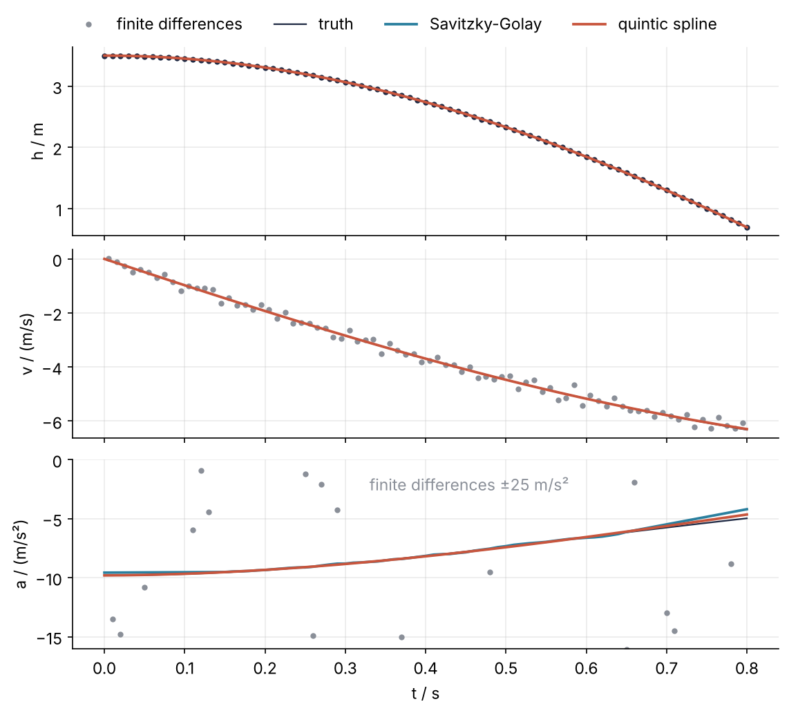
This is where we end up, for a table-tennis ball that air drag slows down: the spline's acceleration follows the true one as it eases from 9.8 to 5 m/s², while the finite differences scatter off the panel. The spline is fitted once to the heights and differentiated twice.

Setup

Two balls, dropped from 3.5 m: a steel ball for which drag is negligible, and a table-tennis ball with quadratic drag and a terminal speed of 9 m/s, whose height has a closed form. Both get Gaussian noise of 1 mm from one seeded generator.

import warnings

import numpy as np
import matplotlib.pyplot as plt
from scipy.interpolate import make_smoothing_spline, make_splrep
from scipy.signal import savgol_filter

g = 9.81          # m/s^2
dt = 0.01         # s, 100 frames per second
sigma = 1e-3      # m, tracking error per frame
h0 = 3.5          # m, release height
v_t = 9.0         # m/s, terminal speed of the table-tennis ball

plt.rcParams.update({
    "figure.figsize": (7, 3.6), "figure.dpi": 110,
    "axes.spines.top": False, "axes.spines.right": False,
    "axes.grid": True, "grid.alpha": 0.25,
    "font.size": 11, "lines.linewidth": 1.8,
})
INK, ACCENT, SECOND, MUTED = "#1f2a44", "#c8553d", "#2a7f9e", "#8a8f98"

t = np.arange(81) * dt
n = t.size
rng = np.random.default_rng(2026)

# steel ball, free fall
h_free_true = h0 - 0.5 * g * t**2
h_free = h_free_true + rng.normal(0, sigma, n)

# table-tennis ball, quadratic drag, exact solution
x = g * t / v_t
h_drag_true = h0 - v_t**2 / g * np.log(np.cosh(x))
v_drag_true = -v_t * np.tanh(x)
a_drag_true = -g / np.cosh(x) ** 2
h_drag = h_drag_true + rng.normal(0, sigma, n)

rms = lambda e: np.sqrt(np.mean(np.square(e)))
mid = slice(5, -5)                       # 50 to 750 ms, away from both ends

a_fd = np.diff(h_free, 2) / dt**2
print(f"{n} heights; second difference: mean {a_fd.mean():.1f} m/s², std {a_fd.std():.1f} m/s²")

81 heights; second difference: mean -9.7 m/s², std 25.0 m/s²

Step 1: Fit a smoothing spline to the positions

A spline is a chain of polynomial pieces, cubic here, joined at points called knots so that value, slope, and curvature are continuous across each joint. A smoothing spline does not pass through the data. make_smoothing_spline puts a knot at every sample and finds the curve \(f\) that minimizes

closeness to the data \(y_i\) against bending, with weights \(w_i\) that default to one. The parameter \(\lambda\) decides between the two. Leave it out, and the function picks it by generalized cross-validation (GCV). Plain cross-validation would leave each point out in turn, predict it from the others, and keep the \(\lambda\) that predicts best. GCV approximates that score from one fit per \(\lambda\): it divides the residual by how much freedom the fit has left, so a \(\lambda\) that buys a small residual by chasing the noise gains nothing.

spl = make_smoothing_spline(t, h_free)
resid = h_free - spl(t)
print(type(spl).__name__, "with", len(spl.t), "knots, degree", spl.k)
print(f"rms residual {1e3 * rms(resid):.2f} mm   (noise σ = {1e3 * sigma:.0f} mm)")

BSpline with 87 knots, degree 3
rms residual 0.86 mm   (noise σ = 1 mm)

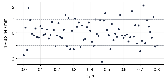
The result is a BSpline, called like a function. spl.t is its knot vector: the 81 sample times with each end time repeated until it appears k + 1 = 4 times, 87 entries in all, a storage habit of B-splines that Step 4 relies on. The residuals are 0.86 mm rms, just under the noise of 1 mm. The spline follows the fall and leaves the noise behind.

Copy

fig, ax = plt.subplots(figsize=(7, 3))
ax.plot(t, 1e3 * resid, "o", color=INK, ms=4)
for level in (-1, 1):
    ax.axhline(level, color=MUTED, lw=1, ls="--")
ax.set(xlabel="t / s", ylabel="h − spline / mm")
plt.show()

Step 2: Too little and too much smoothing

To see what GCV chose, set lam by hand. The data are synthetic, so each fit gets two numbers: its distance from the data, and from the true curve.

print(" lambda / s³   residual / mm   error vs truth / mm")
for lam in [1e-9, 1e-7, 1e-6, 1e-5, 1e-3, 1e-2]:
    s = make_smoothing_spline(t, h_free, lam=lam)
    print(f"   {lam:7.0e}      {1e3 * rms(h_free - s(t)):6.2f}          {1e3 * rms(h_free_true - s(t)):6.2f}")
print(f"   {'GCV':>7s}      {1e3 * rms(resid):6.2f}          {1e3 * rms(h_free_true - spl(t)):6.2f}")

 lambda / s³   residual / mm   error vs truth / mm
     1e-09        0.02            1.01
     1e-07        0.51            0.73
     1e-06        0.73            0.61
     1e-05        0.91            0.63
     1e-03        6.91            6.95
     1e-02       29.45           29.43
       GCV        0.86            0.59

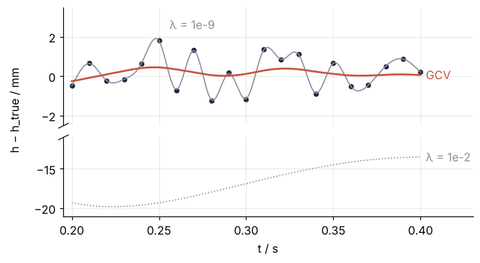
A small \(\lambda\) runs through the points and keeps the noise whole: 0.02 mm from the data, 1.01 mm from the truth. A large one bends 29 mm away from the parabola. GCV does not report its \(\lambda\), but its residual of 0.86 mm places it between the rows for 1e-6 and 1e-5, and its error of 0.59 mm is the lowest in the table. Real data have no truth column; Step 6 gives the rule for them.

The data term is in m² and the curvature integral in m²/s³, so \(\lambda\) is in s³. Count time in milliseconds and the same fit needs a \(\lambda\) \(10^9\) times larger: a value from one data set does not carry over to the next.

Copy

zoom = (t >= 0.2) & (t <= 0.4)
t_fine = np.linspace(0.2, 0.4, 400)
h_fine_true = h0 - 0.5 * g * t_fine**2
s_lo = make_smoothing_spline(t, h_free, lam=1e-9)
s_hi = make_smoothing_spline(t, h_free, lam=1e-2)
dev = lambda f: 1e3 * (f(t_fine) - h_fine_true)          # deviation from the truth in mm

# a broken y axis: the near curves on top, the far one below
fig, (ax, ax_lo) = plt.subplots(2, 1, figsize=(7, 3.6), sharex=True,
                                gridspec_kw=dict(height_ratios=[3, 2], hspace=0.12))
ax.plot(t[zoom], 1e3 * (h_free - h_free_true)[zoom], "o", color=INK, ms=4)
ax.plot(t_fine, dev(s_lo), color=MUTED, lw=1.1)
ax.plot(t_fine, dev(spl), color=ACCENT)
ax_lo.plot(t_fine, dev(s_hi), color=MUTED, lw=1.1, ls=":")
ax.text(0.403, dev(spl)[-1], "GCV", color=ACCENT, va="center")
ax.text(0.256, 2.4, "λ = 1e-9", color=MUTED)
ax_lo.text(0.403, dev(s_hi)[-1], "λ = 1e-2", color=MUTED, va="center")
ax.set(ylim=(-2.5, 3.5), xlim=(0.195, 0.43))
ax_lo.set(ylim=(-21, -11), xlabel="t / s")
ax.spines["bottom"].set_visible(False)
ax.tick_params(bottom=False)
cut = dict(marker=[(-1, -0.5), (1, 0.5)], ms=10, ls="none", color=INK, mew=1, clip_on=False)
ax.plot([0], [0], transform=ax.transAxes, **cut)
ax_lo.plot([0], [1], transform=ax_lo.transAxes, **cut)
fig.supylabel("h − h_true / mm", fontsize=11)
plt.show()

Step 3: Differentiate the spline

A spline's derivative is again a spline, one degree lower, and derivative(nu) returns the nu-th one. Velocity and acceleration are two calls away:

v_spl = spl.derivative()(t)
a_spl = spl.derivative(2)(t)

v_fd = np.diff(h_free) / dt                # first difference, at the midpoints
t_fd = t[:-1] + dt / 2
print(f"velocity rms error: spline {rms(v_spl + g * t):.3f} m/s, first difference {rms(v_fd + g * t_fd):.3f} m/s")
print(f"acceleration 50 to 750 ms: mean {a_spl[mid].mean():.2f} m/s², rms error {rms(a_spl[mid] + g):.2f} m/s²")
print("first six values / (m/s²):", np.round(a_spl[:6], 2) + 0.0)

stiff = make_smoothing_spline(t, h_free, lam=3e-5)
a_stiff = stiff.derivative(2)(t)
print(f"lam=3e-5: residual {1e3 * rms(h_free - stiff(t)):.2f} mm, acceleration rms error {rms(a_stiff[mid] + g):.2f} m/s², "
      f"end values {abs(a_stiff[0]):.2f} and {abs(a_stiff[-1]):.2f} m/s²")

velocity rms error: spline 0.037 m/s, first difference 0.141 m/s
acceleration 50 to 750 ms: mean -9.86 m/s², rms error 1.00 m/s²
first six values / (m/s²): [  0.    -2.77  -4.91  -9.15 -10.39 -10.08]
lam=3e-5: residual 1.15 mm, acceleration rms error 0.48 m/s², end values 0.00 and 0.00 m/s²

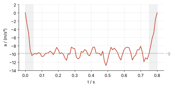
The velocity is four times better than the first difference, 0.037 against 0.141 m/s. The acceleration averages 9.86 m/s² in magnitude, but its rms error is 1.0 m/s², and the first values climb from exactly zero. The second derivative of a cubic is piecewise linear, so the acceleration is a polyline through the noise. The zeros come from the penalty in Step 1: \(\int f''^2\) is smallest when the curvature vanishes wherever no data hold it, so beyond the first and last sample the fit is a straight line, and \(f''\) is zero at both ends. That is the natural spline, and its pull reaches about 40 ms into the data. A stiffer fit, lam=3e-5, raises the residual from 0.86 to 1.15 mm and halves the interior error of the acceleration. Its ends stay at zero.

Copy

fig, ax = plt.subplots(figsize=(7, 3.2))
for span in [(0, 0.05), (0.75, 0.8)]:
    ax.axvspan(*span, color=MUTED, alpha=0.12, lw=0)
ax.axhline(-g, color=MUTED, lw=1, ls="--")
ax.plot(t, a_spl, color=ACCENT)
ax.text(1.01, -g, "−g", color=MUTED, va="center", transform=ax.get_yaxis_transform())   # just right of the axes
ax.set(xlabel="t / s", ylabel="a / (m/s²)", ylim=(-14, 2))
plt.show()

The cubic smoothing spline is the right tool for positions and velocity and a coarse one for acceleration.