Floating-point numbers: why 0.1 + 0.2 is not 0.3, and a derivative's best step

The question

Ask Python whether 0.1 + 0.2 equals 0.3:

import math
import struct
from decimal import Decimal
from fractions import Fraction

import numpy as np
import matplotlib.pyplot as plt

plt.rcParams.update({
    "figure.figsize": (7, 3.6), "figure.dpi": 110,
    "axes.spines.top": False, "axes.spines.right": False,
    "axes.grid": True, "grid.alpha": 0.25,
    "font.size": 11, "lines.linewidth": 1.8,
})
INK, ACCENT, SECOND, MUTED = "#1f2a44", "#c8553d", "#2a7f9e", "#8a8f98"

eps = np.finfo(float).eps
x0 = 1.0
true = np.cos(x0)                      # the exact derivative of sin at x0


def digits(approx):
    """Correct digits: minus log10 of the relative error against cos(1)."""
    return -np.log10(np.abs(approx - true) / abs(true))


def forward(h):
    return (np.sin(x0 + h) - np.sin(x0)) / h


def central(h):
    return (np.sin(x0 + h) - np.sin(x0 - h)) / (2 * h)


print(0.1 + 0.2)
print(0.1 + 0.2 == 0.3)

0.30000000000000004
False

The sum prints as 0.30000000000000004 and the comparison fails. Most people meet this in their first week of programming and learn only that floating-point numbers are "not exact".

The same rounding costs results in places where nobody prints the seventeenth digit. Take the derivative of sin at x = 1, which is cos 1 = 0.5403023058681398, and estimate it the way every textbook starts, with the forward difference

where the step h is the distance between the two points. Calculus says that the smaller h, the closer D(h) comes to cos 1. Measure how close in correct digits, minus the base-10 logarithm of the relative error, so that 3 correct digits is an error of one part in a thousand. Here they are for steps from 10⁻¹ down to 10⁻¹⁴:

Show code

Copy

h = 10.0 ** -np.arange(1, 15)
d = digits(forward(h))
print(f"cos(1) = {float(true)!r}")
for row in [slice(0, 7), slice(7, 14)]:
    print("step h        " + "".join(f"{v:7.0e}" for v in h[row]))
    print("correct digits" + "".join(f"{v:7.2f}" for v in d[row]))

fig, ax = plt.subplots(figsize=(7, 3.4))
ax.plot(h, d, "o-", color=ACCENT, lw=1.2, ms=6)
ax.axvline(1e-8, color=MUTED, lw=1, ls="--")
ax.annotate(f"{d[7]:.1f} digits at h = 10⁻⁸", (1e-8, d[7]), xytext=(12, 0),
            textcoords="offset points", va="center", color=ACCENT)
ax.set(xscale="log", xlabel="step h", ylabel="correct digits", ylim=(0, 9.5))
plt.show()

cos(1) = 0.5403023058681398
step h          1e-01  1e-02  1e-03  1e-04  1e-05  1e-06  1e-07
correct digits   1.10   2.11   3.11   4.11   5.11   6.11   7.11
step h          1e-08  1e-09  1e-10  1e-11  1e-12  1e-13  1e-14
correct digits   8.26   7.01   6.97   5.66   4.10   2.87   2.16

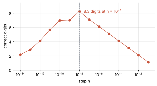
Read from the right, the curve does what calculus promises. Each decade of smaller step buys one more correct digit, from 1.1 at h = 10⁻¹ to 8.3 at 10⁻⁸. Then the curve turns around. At 10⁻¹² only 4.1 digits are left, the same as at 10⁻⁴, and at 10⁻¹⁴ the estimate is down to 2.2.

No formula in a calculus book makes a smaller step worse. So why does it get worse here, and which step is best? The answer is the rounding behind 0.30000000000000004, and once you see it, both puzzles are the same puzzle.

The idea: every number is rounded to 53 binary digits

A floating-point number, a float for short, stores a value as a binary fraction with 53 significant bits, times a power of two. Fifty-three bits are about 16 decimal digits. Any number that needs more is rounded to the nearest one that fits.

Most decimal fractions need more, infinitely more. Binary digits after the point stand for 1/2, 1/4, 1/8, and so on, and one tenth is no finite sum of those: in binary it is 0.0001100110011..., with the block 0011 repeating forever, as 1/3 = 0.333... repeats in decimal. The computer keeps 53 significant bits and rounds the rest away. Python's decimal module prints the exact value that ends up stored:

for text, v in [("0.1", 0.1), ("0.2", 0.2), ("0.3", 0.3), ("0.1 + 0.2", 0.1 + 0.2)]:
    print(f"{text:9s} is stored as {Decimal(v)}")
print(f"\nstored 0.1 - 1/10 = {float(Fraction(0.1) - Fraction(1, 10)):+.3g}")
print(f"stored 0.3 - 3/10 = {float(Fraction(0.3) - Fraction(3, 10)):+.3g}")

below, above = 0.3, np.nextafter(0.3, 1)        # float(0.3) and the next float up
exact = Fraction(0.1) + Fraction(0.2)           # the exact sum of the stored 0.1 and 0.2, drawn next
print(f"\nspacing of the floats near 0.3:    {above - below:.3g}")

0.1       is stored as 0.1000000000000000055511151231257827021181583404541015625
0.2       is stored as 0.200000000000000011102230246251565404236316680908203125
0.3       is stored as 0.299999999999999988897769753748434595763683319091796875
0.1 + 0.2 is stored as 0.3000000000000000444089209850062616169452667236328125

stored 0.1 - 1/10 = +5.55e-18
stored 0.3 - 3/10 = -1.11e-17

spacing of the floats near 0.3:    5.55e-17

The stored 0.1 is 5.55 × 10⁻¹⁸ too large. The stored 0.2 is the same bit pattern one power of two up, so it is too large by twice as much, and the stored 0.3 is 1.11 × 10⁻¹⁷ too small. Near 0.3 the floats sit 5.55 × 10⁻¹⁷ apart, and nothing in between exists:

Show code

Copy

unit = Fraction(1, 10**17)
pos = lambda v: float((Fraction(v) - Fraction(3, 10)) / unit)
grid = [0.3]
for _ in range(3):
    grid = [np.nextafter(grid[0], 0)] + grid + [np.nextafter(grid[-1], 1)]

fig, ax = plt.subplots(figsize=(7, 2.0))
ax.axhline(0, color=MUTED, lw=1, zorder=0)
for g in grid:
    ax.plot([pos(g)] * 2, [-0.25, 0.25], color=MUTED, lw=1.2)
ax.plot([0, 0], [-0.3, 0.55], color=MUTED, lw=1, ls="--")
ax.text(0, 0.6, "0.3", ha="center", va="bottom", color=MUTED)
ax.plot(pos(0.3), 0, "o", color=INK, ms=7, zorder=3)
ax.plot(pos(0.1 + 0.2), 0, "o", color=ACCENT, ms=7, zorder=3)
ax.plot(pos(exact), 0, "o", mfc="white", mec=MUTED, ms=6, zorder=3)
ax.text(pos(0.3), -0.45, "float(0.3)", ha="center", va="top", color=INK)
ax.text(pos(0.1 + 0.2), -0.45, "0.1 + 0.2", ha="center", va="top", color=ACCENT)
ax.plot([pos(exact)] * 2, [0.14, 0.98], color=MUTED, lw=0.8)    # leader straight up from the open circle
ax.text(pos(exact) - 0.25, 1.12, "exact sum of the stored 0.1 and 0.2", ha="left", va="center", color=MUTED)
ax.annotate("", (pos(grid[1]), 0.45), (pos(grid[2]), 0.45),
            arrowprops=dict(arrowstyle="<->", color=MUTED, lw=1, shrinkA=0, shrinkB=0))
ax.text((pos(grid[1]) + pos(grid[2])) / 2, 0.55, "5.55 × 10⁻¹⁷", ha="center", va="bottom", color=MUTED)
ax.set(xlabel="x − 0.3 / 10⁻¹⁷", xlim=(-20, 20), ylim=(-1.1, 1.35), yticks=[])
ax.spines["left"].set_visible(False)
ax.grid(False)
plt.show()

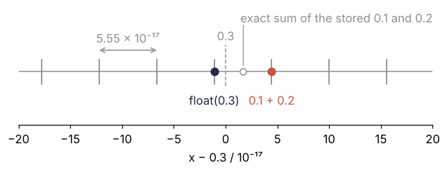
Add the stored 0.1 and the stored 0.2 exactly and you land on the open circle. The result has to be one of the two floats beside it. Here are its distances to both, and the last binary digit of each:

last_bit = lambda v: struct.unpack("<q", struct.pack("<d", v))[0] & 1
print(f"exact sum minus float(0.3):        {float(exact - Fraction(below)):.3g}")
print(f"next float above 0.3 minus sum:    {float(Fraction(above) - exact):.3g}")
print(f"last bit of float(0.3): {last_bit(below)}, of the next float: {last_bit(above)}")

exact sum minus float(0.3):        2.78e-17
next float above 0.3 minus sum:    2.78e-17
last bit of float(0.3): 1, of the next float: 0

The open circle sits 2.78 × 10⁻¹⁷ from each: exactly halfway. A tie goes to the neighbor whose last bit is 0. The rule is called round half to even, and it exists because always rounding ties up would push long sums upward. Here the even neighbor is the upper one, so 0.1 + 0.2 lands one spacing above float(0.3), and the comparison fails by the smallest amount by which it can fail.

Every arithmetic operation rounds its result like this, once, to the nearest float. A single rounding is harmless, but a sum of a million terms collects a million of them.

Now the derivative. sin(1 + h) and sin(1) are each rounded to about 16 digits, and for a small step they share their leading digits, about 4 of them at h = 10⁻⁴, 8 at 10⁻⁸, and 12 at 10⁻¹². The subtraction removes the shared digits and leaves only those in which the two differ, about 16 − 8 = 8 at h = 10⁻⁸ and about 4 at 10⁻¹². Losing digits by subtracting two nearly equal numbers is called catastrophic cancellation. Here it is digit by digit at the three steps:

Show code

Copy

ROWS = ["sin(1 + h)", "sin(1)", "difference", "quotient", "cos(1)"]


def strip(h):
    """The rows of the digit strip at step h: (label, 19 characters, one color per character)."""
    hi, lo = np.sin(x0 + h), np.sin(x0)
    diff = hi - lo
    quot = diff / h
    s_diff = f"{diff:.17f}"
    zeros = len(s_diff[2:]) - len(s_diff[2:].lstrip("0"))      # decimals the subtraction turned to 0
    s_quot, s_true = f"{quot:.17f}", f"{true:.17f}"
    good = 0                                                    # leading decimals that agree with cos(1)
    while good < len(s_true) - 2 and s_quot[2 + good] == s_true[2 + good]:
        good += 1
    rows = []
    for label, s in zip(ROWS, [f"{hi:.17f}", f"{lo:.17f}", s_diff, s_quot, s_true]):
        colors = [INK] * len(s)
        if label == "difference":
            colors = [INK, INK] + [MUTED] * zeros + [INK] * (len(s) - 2 - zeros)
        elif label == "quotient":
            colors = [ACCENT] * (2 + good) + [MUTED] * (len(s) - 2 - good)
        rows.append((label, s, colors))
    return rows, zeros, digits(quot)


# one table in inch coordinates: the row labels once, then one column of digits per step
PITCH, GAP, COL0 = 0.1, 0.35, 1.0                  # inches per character, between columns, labels' width
width, height = COL0 + 3 * 19 * PITCH + 2 * GAP + 0.05, 2.05
fig = plt.figure(figsize=(width, height))
ax = fig.add_axes([0, 0, 1, 1])
ax.set_axis_off()
ax.set(xlim=(0, width), ylim=(height, 0))
row_y = 0.82 + 0.27 * np.arange(len(ROWS))
for label, y in zip(ROWS, row_y):
    ax.text(0.02, y, label, va="center", color=INK)
for j, (k, sup) in enumerate([(4, "⁻⁴"), (8, "⁻⁸"), (12, "⁻¹²")]):
    h = 10.0**-k
    rows, zeros, d = strip(h)
    shared = -np.log10(abs(np.sin(x0 + h) - np.sin(x0)) / np.sin(x0))
    print(f"h = 1e-{k:02d}: shared leading digits {shared:5.2f}, correct digits {d:5.2f}")
    left = COL0 + j * (19 * PITCH + GAP)
    ax.text(left, 0.17, f"h = 10{sup}", va="center", color=INK)
    ax.text(left, 0.44, f"{zeros} cancel, {d:.1f} correct", va="center", color=INK)
    for (label, s, colors), y in zip(rows, row_y):
        for i, (ch, c) in enumerate(zip(s, colors)):
            ax.text(left + PITCH * (i + 0.5), y, ch, va="center", ha="center", family="monospace", color=c)
plt.show()

h = 1e-04: shared leading digits  4.19, correct digits  4.11
h = 1e-08: shared leading digits  8.19, correct digits  8.26
h = 1e-12: shared leading digits 12.19, correct digits  4.10

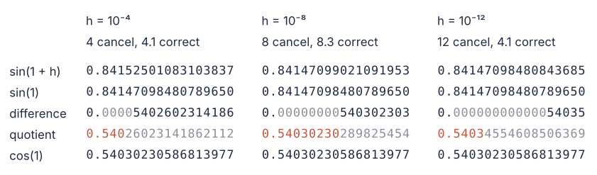
Red marks the quotient digits that agree with cos 1. At 10⁻⁴ there are three, one fewer than the 4.1 correct digits in the header, because the two count different things. Correct digits measure the size of the error, and 0.54026 is off from 0.54030 by less than one part in ten thousand. Matching digits only compare characters, and a quotient that approaches 0.5403023… from below keeps a 2 in its fourth decimal until it reaches 0.5403. At 10⁻⁸ the difference begins after eight zeros, and the quotient's first eight digits match cos 1. At 10⁻¹² twelve zeros leave five digits, the last of them already wrong, and the quotient keeps 4.1 correct. The strip at 10⁻⁴ is the odd one out: only four digits cancel and about twelve survive the subtraction, yet the quotient is correct to just 4.1 digits. That loss is not cancellation.

Two errors that cross

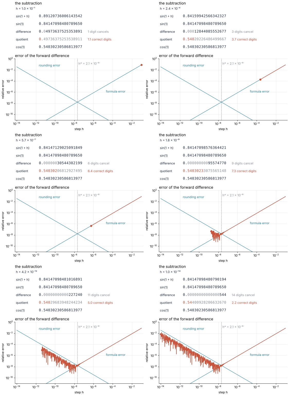
The 10⁻⁴ strip shows the other error. With a large step the formula itself is wrong: the line through two points of the sine is a secant, not the tangent, and its slope differs from cos 1 by an amount proportional to h. At h = 10⁻⁴ that costs four digits, however exactly the arithmetic is done.

The rounding error runs the other way. Each sine is off by up to about 10⁻¹⁶ of its size, half of a number called machine epsilon, ε, which the next section pins down. The quotient divides that by h, and 10⁻¹⁶ / 10⁻⁸ = 10⁻⁸ is the eight digits counted above. So the formula error shrinks like h and the rounding error grows like ε/h. Sweep the step from 10⁻¹ down to 10⁻¹⁴ and watch both:

How I built this: Matplotlib animation with FuncAnimation: a probe sweep as a small GIF.

Coming in from the right, the measured error follows the formula-error line down, one decade per decade. Near h = 2 × 10⁻⁸ it meets the rounding line and turns into a jagged band that climbs back up along it. The jags are rounding as well: whether the last bits of sin(1 + h) happen to round in your favor for one particular h is chance, and the next h may be unlucky. The best step is therefore where the two lines cross, not the lowest jag.

Formalization

A double-precision float, the default in Python and NumPy, has 64 bits: 1 sign bit s, 11 exponent bits e, and 52 fraction bits m. They stand for

The leading 1 is not stored, since every nonzero binary number starts with one, so the significand carries 53 bits for the price of 52. The stored exponent e is shifted by 1023 so that it needs no sign of its own. Its end values, 0 and 2047, are reserved for zero, infinity, and other special cases. The rest, the normal floats, span powers of two from −1022 to 1023. Here is 0.1:

bits = format(struct.unpack(">Q", struct.pack(">d", 0.1))[0], "064b")
e = int(bits[1:12], 2)
print(f"sign      {bits[0]}")
print(f"exponent  {bits[1:12]} = {e}, so the power of two is {e} - 1023 = {e - 1023}")
print(f"fraction  {bits[12:]}")
print(f"hex       {(0.1).hex()}")
print(f"powers of two in normal floats: {np.finfo(float).minexp} to {np.finfo(float).maxexp - 1}")

sign      0
exponent  01111111011 = 1019, so the power of two is 1019 - 1023 = -4
fraction  1001100110011001100110011001100110011001100110011010
hex       0x1.999999999999ap-4
powers of two in normal floats: -1022 to 1023

So 0.1 = 1.6 × 2⁻⁴. Normalizing moves the binary point past the first 1, so the fraction reads the 0011 cycle of the previous section as 1001. The cycle would have put 1001 in the last four places, but the bits after them begin with a 1, more than half, so the fraction is rounded up to end in 1010. That rounding is the 5.55 × 10⁻¹⁸.

Three consequences follow, and you need them whenever a number looks wrong.

print(f"eps = 2**-52           {eps:.3g}   {eps == 2.0**-52}")
print(f"largest rounding, eps/2 {eps / 2:.3g}")
print(f"decimal digits in 53 bits: {53 * math.log10(2):.2f}; safe round trip: {np.finfo(float).precision}")
print(f"0.1 + 0.2 to 16 digits: {0.1 + 0.2:.16g}, to 17 digits: {0.1 + 0.2:.17g}")
print(f"printed by Python: 0.1 as {0.1!r}, 0.1 + 0.2 as {0.1 + 0.2!r}")
for x in [0.3, 1e8, 1e16]:
    print(f"spacing at {x:5.0e}: {np.spacing(x):.3g}")
print(f"1e16 + 1 == 1e16: {1e16 + 1 == 1e16}")

eps = 2**-52           2.22e-16   True
largest rounding, eps/2 1.11e-16
decimal digits in 53 bits: 15.95; safe round trip: 15
0.1 + 0.2 to 16 digits: 0.3, to 17 digits: 0.30000000000000004
printed by Python: 0.1 as 0.1, 0.1 + 0.2 as 0.30000000000000004
spacing at 3e-01: 5.55e-17
spacing at 1e+08: 1.49e-08
spacing at 1e+16: 2
1e16 + 1 == 1e16: True

Machine epsilon and the digits a float carries. The gap between 1 and the next float is ε = 2⁻⁵² = 2.22 × 10⁻¹⁶, NumPy's np.finfo(float).eps. Rounding to the nearest float changes a number by at most half a gap, ε/2 = 1.11 × 10⁻¹⁶ of its size. Fifty-three bits make 15.95 decimal digits: any decimal number with 15 significant digits survives the trip into a float and back unchanged, and 17 digits are needed to tell every float apart. Python prints the shortest decimal that reads back as the same float: 0.1 for the stored 0.1, and 17 digits for 0.1 + 0.2, because at 16 it would read 0.3, a different float.

The spacing grows with the number. The gap at x is about ε|x|: 5.55 × 10⁻¹⁷ at 0.3, 1.49 × 10⁻⁸ at 10⁸, and 2 at 10¹⁶, where 1e16 + 1 == 1e16 is True. An absolute tolerance of 10⁻¹⁰ near 10⁸ asks for a precision over a hundred times finer than the floats there have. Tolerances must be relative.

A difference quotient has a best step. Correctly rounded, f(x + h) and f(x) are each off by up to ε|f|/2, so their difference is off by up to ε|f|, and dividing by h gives a rounding error of ε|f|/h. Taylor's theorem, f(x + h) = f(x) + h f'(x) + (h²/2) f''(x) + …, gives the formula's error, (h/2)|f''|. Together,

with the best step h* where E is smallest, exactly where its two terms are equal. For sin, f'' = −sin, so |f/f''| = 1 at every x and h* = √(2ε) = 2.1 × 10⁻⁸. The model predicts 7.5 correct digits there, the measurement 7.9. The central difference (f(x + h) − f(x − h))/(2h) does better: the second-order terms of the two Taylor expansions cancel, so the error starts at the third-order term,

For sin at 1, f''' = −cos, so h* = (1.5 ε tan 1)^(1/3) = 8.0 × 10⁻⁶, with 10.5 digits predicted and 11.7 measured.

You rarely know f'' or f''', so take the ratios as one and drop the small constants. Use a step of √ε = 1.5 × 10⁻⁸ for forward differences and ε^(1/3) = 6.1 × 10⁻⁶ for central ones, times max(|x|, 1). The factor makes the step relative to x, as tolerances are: at x = 3000 it is 3000 times the step at x = 1. Near x = 0 the floor of 1 keeps the step from vanishing, which assumes a unit in which your values are of order one. SciPy's approx_derivative uses exactly these steps and this factor.

Show code

Copy

f, f2, f3 = np.sin(x0), np.sin(x0), np.cos(x0)       # |f|, |f''|, |f'''| for sin at x0
E_fwd = lambda h: h / 2 * f2 + eps * f / h            # the two error models
E_cen = lambda h: h**2 / 6 * f3 + eps * f / (2 * h)
h_fwd = np.sqrt(2 * eps * f / f2)
h_cen = (3 * eps * f / (2 * f3)) ** (1 / 3)
for name, method, E, hs in [("forward", forward, E_fwd, h_fwd), ("central", central, E_cen, h_cen)]:
    print(f"{name}: h* = {hs:.1e}, model {-np.log10(E(hs) / true):.1f} digits, measured {digits(method(hs)):.1f}")

h = np.logspace(-14, -1, 261)
err_fwd, err_cen = np.abs(forward(h) - true) / true, np.abs(central(h) - true) / true
model_fwd, model_cen = E_fwd(h) / true, E_cen(h) / true          # relative, like the measurement
worst = max((err_fwd / model_fwd).max(), (err_cen / model_cen).max())
print(f"measurement above model by at most {100 * (worst - 1):.1f} %")
print(f"central h* / forward h* = {h_cen / h_fwd:.0f}")


def sci(v):
    """2.1e-08 as '2.1 × 10⁻⁸'."""
    mant, ex = f"{v:.1e}".split("e")
    return f"{mant} × 10" + str(int(ex)).translate(str.maketrans("-0123456789", "⁻⁰¹²³⁴⁵⁶⁷⁸⁹"))


fig, axes = plt.subplots(2, 1, figsize=(7, 4.4), sharex=True)
for ax, err, model, hs, name in [(axes[0], err_fwd, model_fwd, h_fwd, "forward difference"),
                                 (axes[1], err_cen, model_cen, h_cen, "central difference")]:
    ax.plot(h, model, color=SECOND, lw=1.1)
    ax.plot(h, err, color=ACCENT, lw=1.4)
    ax.axvline(hs, color=MUTED, lw=1, ls="--")
    ax.text(hs * 1.4, 1e-1, f"h* = {sci(hs)}", color=MUTED, va="top")
    ax.text(0.02, 0.06, name, transform=ax.transAxes, color=INK)
    ax.set(yscale="log", ylabel="relative error", ylim=(1e-13, 1))
axes[0].text(3e-12, 3e-3, "model", color=SECOND, ha="center", va="bottom")
axes[0].text(3e-12, 3e-8, "measured", color=ACCENT, ha="center", va="top")
axes[1].set(xscale="log", xlabel="step h")
plt.show()

forward: h* = 2.1e-08, model 7.5 digits, measured 7.9
central: h* = 8.0e-06, model 10.5 digits, measured 11.7
measurement above model by at most 2.1 %
central h* / forward h* = 381

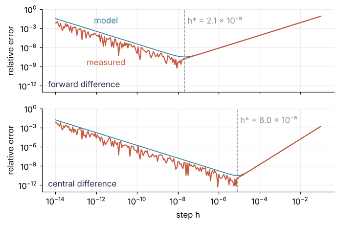
The measured curves rise at most 2.1 % above the model, so the model bounds the error to a good approximation, and the jags below it are rounding that happened to cancel. The central difference wins by three digits in the model and nearly four in the measurement, at a step 381 times larger.

See it in code

The standard calls for all of the above are NumPy's finfo, spacing, and nextafter, and math from the standard library. np.nextafter(a, b) returns the next float after a in the direction of b; the second argument only gives the direction.

print(f"machine epsilon                   {float(np.finfo(float).eps)!r}")
print(f"spacing above 0.3                 {float(np.nextafter(0.3, 1) - 0.3)!r}")
print(f"0.1 + 0.2 == next float above 0.3 {0.1 + 0.2 == np.nextafter(0.3, 1)}")
print(f"math.isclose(0.1 + 0.2, 0.3)      {math.isclose(0.1 + 0.2, 0.3)}")
print(f"math.isclose(1e-20, 0.0)          {math.isclose(1e-20, 0.0)}")

total = 0.0
for _ in range(1_000_000):             # a plain loop: one rounding per addition
    total += 0.1
print(f"\n0.1 added 10**6 times in a loop   {total!r}")
print(f"math.fsum of the same             {math.fsum([0.1] * 1_000_000)!r}")
print(f"built-in sum of the same          {sum([0.1] * 1_000_000)!r}")
print(f"math.fsum([0.1, 0.2])             {math.fsum([0.1, 0.2])!r}")
print(f"sum, fsum of [1, 2**-53, 2**-106] {sum([1.0, 2**-53, 2**-106])!r}, {math.fsum([1.0, 2**-53, 2**-106])!r}")

print(f"\nforward, h = sqrt(eps) = {np.sqrt(eps):.2g}  {forward(np.sqrt(eps)):.16f}  {digits(forward(np.sqrt(eps))):5.2f} digits")
print(f"central, h = eps**(1/3) = {eps ** (1 / 3):.2g} {central(eps ** (1 / 3)):.16f}  {digits(central(eps ** (1 / 3))):5.2f} digits")
print(f"cos(1)                           {true:.16f}")

machine epsilon                   2.220446049250313e-16
spacing above 0.3                 5.551115123125783e-17
0.1 + 0.2 == next float above 0.3 True
math.isclose(0.1 + 0.2, 0.3)      True
math.isclose(1e-20, 0.0)          False

0.1 added 10**6 times in a loop   100000.00000133288
math.fsum of the same             100000.0
built-in sum of the same          100000.0
math.fsum([0.1, 0.2])             0.30000000000000004
sum, fsum of [1, 2**-53, 2**-106] 1.0, 1.0000000000000002

forward, h = sqrt(eps) = 1.5e-08  0.5403022989630699   7.89 digits
central, h = eps**(1/3) = 6.1e-06 0.5403023058631032  11.03 digits
cos(1)                           0.5403023058681398

The loop ends 1.3 × 10⁻⁶ above 100000, a million roundings that mostly leaned the same way. math.fsum returns the exact sum of the stored values, rounded once, and that is 100000.0. The built-in sum gives 100000.0 as well: on the Python 3.12 that ran this notebook it carries a running correction for the rounding of each addition, Neumaier's method, which is why the drift needs a plain loop to show. The correction is not fsum's exact sum. In 1 + 2⁻⁵³ + 2⁻¹⁰⁶, the 2⁻⁵³ is half the gap at 1, a tie as for 0.1 + 0.2, and the tiny 2⁻¹⁰⁶ tips it upward: fsum returns the correctly rounded 1.0000000000000002, sum returns 1.0. Neither repairs 0.1 + 0.2, because that error sits in the stored 0.1 and 0.2 before any addition happens.

Compare floats with math.isclose, never with ==. Its default tolerance is relative, 10⁻⁹, which is why it fails against zero: give it an abs_tol there. The rule-of-thumb steps land within a digit of what the model's best step gave, 7.89 digits against 7.9 for the forward difference and 11.03 against 11.7 for the central one.

Where it shows up

print(f"sqrt(eps) = {np.sqrt(eps):.4g}, 100 * eps = {100 * eps:.3g}")

rng = np.random.default_rng(1)
x = 1e9 + rng.standard_normal(100_000)          # readings with a large offset and unit scatter
print(f"variance as mean(x**2) - mean(x)**2: {np.mean(x**2) - np.mean(x)**2:.4g}, np.var: {np.var(x):.3g}")

eps32 = np.finfo(np.float32).eps
step32 = float(np.spacing(np.float32(100.0)))
print(f"float32: eps = {eps32:.3g}, spacing at 100 degrees = {step32:.2g} degrees = {step32 * 111.32e3:.2f} m")

b, c = -1e8, 1.0                                # x**2 + b x + c = 0
q = (-b + np.sqrt(b * b - 4 * c)) / 2           # the large root, no cancellation
small_textbook = (-b - np.sqrt(b * b - 4 * c)) / 2
print(f"small root: textbook {small_textbook:.3g} ({100 * (1 - small_textbook / 1e-8):.1f} % off), c/q {c / q:.3g}")

sqrt(eps) = 1.49e-08, 100 * eps = 2.22e-14
variance as mean(x**2) - mean(x)**2: 128, np.var: 0.993
float32: eps = 1.19e-07, spacing at 100 degrees = 7.6e-06 degrees = 0.85 m
small root: textbook 7.45e-09 (25.5 % off), c/q 1e-08

• Chemistry: fitting and optimization. scipy.optimize.minimize given no gradient, which means BFGS for a problem without bounds or constraints, takes forward differences with an absolute step of √ε = 1.49 × 10⁻⁸, and least_squares, which curve_fit calls for a fit with bounds, uses √ε or ε^(1/3) times max(|x|, 1). A rate constant of 10⁻⁹ in your units is therefore stepped by fifteen times its own size, so rescale parameters to order one before you fit (Minimization with scipy.optimize.minimize, Fit a curve to data with error bars).
• Physics and engineering: integrals and ODEs. quad's default tolerances epsabs and epsrel are 1.49 × 10⁻⁸, equal to √ε in three digits. solve_ivp raises any rtol below 100ε = 2.2 × 10⁻¹⁴ to that value with a warning, so no tolerance can ask for more digits than the floats hold (solve_ivp from the ground up).
• Biology: summary statistics. A variance computed as mean(x²) − mean(x)² is catastrophic cancellation whenever the mean is large against the scatter. For 100,000 readings of 10⁹ with a scatter of 1, it gives 128 where np.var, which subtracts the mean first, gives 0.993.
• Geology: coordinates in float32. Rasters and coordinate arrays are often stored in single precision, float32, whose ε is 1.19 × 10⁻⁷. Its spacing at a longitude of 100° is 7.6 × 10⁻⁶ degrees, 0.85 m on the ground at the equator, so storing positions as float32 rounds them to most of a meter.
• Mathematics: the quadratic formula. For x² + bx + c = 0 with b = −10⁸ and c = 1, the textbook formula for the small root, (−b − √(b² − 4c))/2, subtracts two nearly equal numbers and returns 7.45 × 10⁻⁹, 25.5 % off the true 1.0 × 10⁻⁸. The product of the roots is c, so the small root is also c/q with the large root q = (−b + √(b² − 4c))/2, which subtracts nothing and comes out right.

In every case the same two facts carry over: a float holds about 16 significant digits relative to its own size, and every subtraction of nearly equal numbers spends some of them.

Further reading

• D. Goldberg, "What every computer scientist should know about floating-point arithmetic", ACM Computing Surveys (1991), for the format and the rounding rules in full.
• Higham, Accuracy and Stability of Numerical Algorithms, chapter 1, for rounding error as a numerical analyst counts it.
• numpy.finfo for the machine constants of every float type, and the Python tutorial's chapter Floating-Point Arithmetic: Issues and Limitations.
• Related tutorials on this site: Numerical integration with scipy.integrate: the area under a measured peak; solve_ivp from the ground up: the pendulum beyond small angles; Minimization with scipy.optimize.minimize: the shape of a seven-atom cluster; Fit a curve to data with error bars and draw a confidence band; Matplotlib animation with FuncAnimation: a probe sweep as a small GIF, how the animation above was built; planned: Floating-point numbers in Julia.
• Download the notebook. It was executed with the library versions in the header.