Linear ODE systems with SymPy's dsolve: the Bateman function of an oral dose

The problem: how high does a drug level climb with a tablet every 8 hours?

A tablet of 500 mg dissolves in the gut, and the drug passes into the blood at a first-order rate of \(k_a = 1.0\) /h. The body clears it at \(k_e = 0.2\) /h, a half-life of 3.47 h. After one tablet the plasma level peaks 2.0 h later at 6.7 mg/L. Take one every 8 hours and each tablet lands on what is left of the one before, until the level swings between a trough of 3.2 mg/L, the lowest level just before the next tablet, and a peak of 8.9 mg/L. Every one of these numbers comes from a linear ODE system that SymPy's dsolve solves exactly, and the regular schedule then sums in closed form.

The model has two compartments, the gut and the body, and each loses drug at a rate proportional to what it holds:

\(G\) and \(A\) are the amounts of drug in gut and body, and \(D = 500\) mg is the dose, all of it absorbed. The plasma concentration is \(C = A/V\), with \(V = 50\) L the apparent volume of distribution: the volume the drug would fill if it were everywhere at its plasma concentration. The numbers are illustrative and belong to no particular drug. SymPy itself is introduced in SymPy from the ground up.

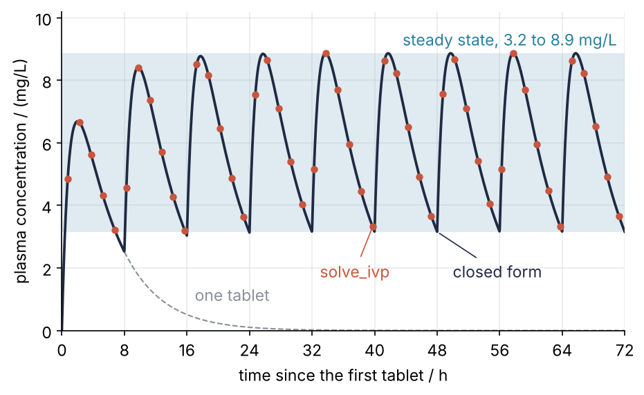
This is where we end up: three days of a tablet every 8 hours. The line is the closed form from dsolve and summation, the dots an independent solve_ivp run, the band the exact steady state. Harry Bateman wrote this solution down in 1910 for chains of radioactive decays, decades before pharmacokinetics borrowed it for the tablet.

Setup

The symbols carry their assumptions from the start, because Step 5 needs them (Pitfall 2 shows what happens without). The numbers are rationals, so every substitution stays exact until a float is asked for.

import warnings
import numpy as np
import sympy as sp
import matplotlib.pyplot as plt
from scipy.integrate import solve_ivp

plt.rcParams.update({
    "figure.figsize": (7, 3.6), "figure.dpi": 110,
    "axes.spines.top": False, "axes.spines.right": False,
    "axes.grid": True, "grid.alpha": 0.25,
    "font.size": 11, "lines.linewidth": 1.8,
})
INK, ACCENT, SECOND, MUTED = "#1f2a44", "#c8553d", "#2a7f9e", "#8a8f98"

t, s = sp.symbols("t s", nonnegative=True)                 # time, time since the last tablet
k_a, k_e, k, D, V, tau = sp.symbols("k_a k_e k D V tau", positive=True)
n = sp.symbols("n", integer=True, positive=True)            # number of tablets taken
j = sp.symbols("j", integer=True, nonnegative=True)         # index of a tablet
G = sp.Function("G")                                        # amount in the gut / mg
A = sp.Function("A")                                        # amount in the body / mg

vals = {k_a: 1, k_e: sp.Rational(1, 5), D: 500, V: 50, tau: 8}   # 1/h, 1/h, mg, L, h

print(f"SymPy {sp.__version__}")

SymPy 1.14.0

Step 1: Write the two compartments as a system of equations

Each compartment loses drug at a rate proportional to its content, the first-order kinetics of radioactive decay or of an enzyme far below saturation. What leaves the gut at the rate \(k_a G\) enters the body, which loses \(k_e A\). In SymPy the unknowns are applied functions, G(t) and A(t), and each equation is an Eq between a derivative and its right-hand side:

eqs = [sp.Eq(G(t).diff(t), -k_a * G(t)),
       sp.Eq(A(t).diff(t), k_a * G(t) - k_e * A(t))]
for eq in eqs:
    print(eq)

Eq(Derivative(G(t), t), -k_a*G(t))
Eq(Derivative(A(t), t), k_a*G(t) - k_e*A(t))

The system is linear with constant coefficients: \(G\) and \(A\) appear only to the first power, multiplied by constants. When the rates differ, the solutions of such a system are sums of exponentials \(e^{\lambda t}\), one for each rate, and that is what dsolve will find.

Step 2: Solve the system with dsolve and its initial values

Without initial values, dsolve takes the list of equations and returns the general solution:

print(sp.dsolve(eqs))

[Eq(G(t), -C1*(k_a - k_e)*exp(-k_a*t)/k_a), Eq(A(t), C1*exp(-k_a*t) + C2*exp(-k_e*t))]

Two constants, C1 and C2, one per equation. In the line for \(A\), C1 multiplies \(e^{-k_a t}\) and C2 multiplies \(e^{-k_e t}\). The gut's line is C1 again, times a factor, because the \(e^{-k_a t}\) part of \(A\) is the only part the gut feeds, so fixing it fixes \(G\). The initial values go into ics, a dict keyed by the functions at \(t = 0\), and the list of functions says which unknowns to solve for:

res = sp.dsolve(eqs, [G(t), A(t)], ics={G(0): D, A(0): 0})
sol = {eq.lhs: eq.rhs for eq in res}
for f in (G(t), A(t)):
    print(f, "=", sol[f])
print(sp.checkodesol(eqs, res))
C = sol[A(t)] / V

G(t) = D*exp(-k_a*t)
A(t) = D*k_a*exp(-k_e*t)/(k_a - k_e) - D*k_a*exp(-k_a*t)/(k_a - k_e)
(True, [0, 0])

The answer is a list of Eq. The dict by left-hand side makes sol[A(t)] the body's amount whatever the order of that list (Pitfall 1). checkodesol substitutes the solution into every equation, derivatives included, which a plain subs does not do, and returns True with one residual per equation, both 0. The gut empties as a plain exponential. The body holds the difference of two exponentials, scaled by \(k_a/(k_a - k_e)\). Divided by \(V\), that is the Bateman function:

Step 3: Find the peak with diff and solve

The peak is where the derivative of \(C\) vanishes:

peak = sp.solve(sp.diff(C, t), t)
print(peak)
t_max = peak[0]
C_max = C.subs(t, t_max)
print(f"t_max = {float(t_max.subs(vals)):.4f} h   C_max = {float(C_max.subs(vals)):.3f} mg/L")

[-log(k_e/k_a)/(k_a - k_e)]
t_max = 2.0118 h   C_max = 6.687 mg/L

Read the answer aloud: \(t_{\max} = \ln(k_a/k_e)/(k_a - k_e)\). The dose and the volume are not in it, so only the two rates decide when the level peaks. The height is evaluated at the numbers and not simplified, because SymPy leaves \(C(t_{\max})\) as exponentials of logarithms that it does not reduce. With the tablet's rates the drug peaks 2.01 h after the tablet, at 6.687 mg/L.

Step 4: Take the case of equal rates with limit

Put \(k_a = k_e\) into the formula and it breaks:

print(C.subs(k_a, k_e))

nan

It is 0/0: the formula divides by \(k_a - k_e\), and the bracket is zero as well. Equal rates are not exotic. Rates fitted to a real drug can come out close to each other, and a scan over \(k_a\) passes through \(k_e\). The curve itself is fine there, and limit finds it:

print(sp.limit(C, k_a, k_e))

D*k_e*t*exp(-k_e*t)/V

The factor \(t\) is new. To see where it comes from, read the bracket over the rate difference, \((e^{-k_e t} - e^{-k_a t})/(k_a - k_e)\), as a difference quotient of the function \(e^{-kt}\) in the rate \(k\), taken between \(k_e\) and \(k_a\). As \(k_a\) approaches \(k_e\) it becomes minus the derivative with respect to \(k\):

print(sp.diff(sp.exp(-k * t), k))

-t*exp(-k*t)

The \(t\) comes from the chain rule. dsolve on the system with one rate \(k\) for both finds the same curve directly:

eqs_k = [eq.subs({k_a: k, k_e: k}) for eq in eqs]
print(sp.dsolve(eqs_k, [G(t), A(t)], ics={G(0): D, A(0): 0}))

[Eq(G(t), D*exp(-k*t)), Eq(A(t), D*k*t*exp(-k*t))]

Only the way the general formula is written breaks at equal rates, and that matters as soon as code evaluates it near them (Pitfall 3).

Step 5: Sum repeated doses with summation and take n to infinity

Each tablet starts its own Bateman curve, and because the system is linear the curves add. With \(s\) the time since the last tablet, the level after \(n\) tablets is

Since \(e^{-k(s + j\tau)} = e^{-ks}\,(e^{-k\tau})^j\), each exponential gives a geometric series in \(j\), and summation returns each series as a Piecewise, a formula that depends on a condition. atoms(sp.Piecewise) collects the Piecewise objects in the result, and has(k_e) picks the one of the elimination term, so that its parts can be printed:

S = sp.summation(C.subs(t, s + j * tau), (j, 0, n - 1))
pw = next(p for p in S.atoms(sp.Piecewise) if p.has(k_e))
print(pw.args)

((n, Eq(exp(-k_e*tau), 1)), ((1 - exp(-k_e*n*tau))/(1 - exp(-k_e*tau)), True))

The parts are (expression, condition) pairs, checked in order. The first pair covers \(e^{-k_e \tau} = 1\), which positive rates and \(\tau\) rule out. The last, with condition True, is the otherwise branch, and it applies here. replace hands every Piecewise its pairs, and the small function returns the expression of the last one:

Cn = S.replace(sp.Piecewise, lambda *pairs: pairs[-1][0])
Css = Cn.subs(n, sp.oo)
print(Css)

D*k_a*exp(-k_e*s)/(V*(1 - exp(-k_e*tau))*(k_a - k_e)) - D*k_a*exp(-k_a*s)/(V*(1 - exp(-k_a*tau))*(k_a - k_e))

Plugging in infinity is safe because \(n\) appears only in \(e^{-k n \tau}\) with \(k\) and \(\tau\) positive, and SymPy knows that \(e^{-\infty} = 0\). Where infinity meets infinity, as in \(\infty - \infty\), subs gives nan, and limit is the tool. The first term carries the accumulation factor \(1/(1 - e^{-k_e \tau})\):

Css_num, C_num = Css.subs(vals), C.subs(vals)
s_peak = sp.solve(sp.diff(Css, s), s)[0].subs(vals)
trough, peak_ss = Css_num.subs(s, 0), Css_num.subs(s, s_peak)
print(f"accumulation factor {float((1 / (1 - sp.exp(-k_e * tau))).subs(vals)):.4f}")
print(f"trough {float(trough):.3f} mg/L = {float(trough / C_num.subs(t, 8)):.4f} x level 8 h after one tablet")
print(f"peak   {float(peak_ss):.3f} mg/L at s = {float(s_peak):.3f} h = {float(peak_ss / C_max.subs(vals)):.4f} x single peak")

accumulation factor 1.2530
trough 3.158 mg/L = 1.2534 x level 8 h after one tablet
peak   8.864 mg/L at s = 1.730 h = 1.3255 x single peak

The factor is 1.253: the trough, 3.158 mg/L, is 1.253 times the level 8 h after the first tablet. Only the elimination term, in \(e^{-k_e s}\), carries the factor, and by then the absorption term has died out, since \(e^{-k_a \tau} = 3.4 \times 10^{-4}\).

The peak rises by a factor of 1.33, to 8.864 mg/L, and comes 1.73 h after the tablet instead of 2.01 h. The peak is where the inflow from the gut equals the elimination from the body. At steady state each interval starts at 3.158 mg/L, so elimination is high from the start and catches up with the falling inflow sooner.