Xenon poisoning with solve_ivp: the xenon peak after a reactor shutdown
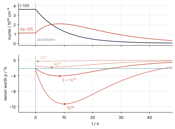
Afterwards you can compute iodine-135 and xenon-135 after a reactor shutdown with solve_ivp and read off the xenon peak, its time, and its reactivity worth.
- Field
- Engineering, Physics
- Libraries
matplotlib 3.11.2numpy 2.5.4scipy 1.18.1
py-xenon-poisoning.ipynb, executed with the versions above. The download needs a free account
Run it yourself. In a terminal, this installs exactly the versions above:
pip install numpy==2.5.4 scipy==1.18.1 matplotlib==3.11.2 jupyterlabThe problem
A reactor has run for days at a thermal flux of 3 × 10¹³ cm⁻² s⁻¹ and shuts down. You want the xenon peak from solve_ivp, its time, and how long it lasts. The flux \(\phi\) counts neutrons through 1 cm² per second. Xenon's cross section \(\sigma_X\), the target area of one nucleus, makes \(\sigma_X\phi X\) absorptions per cm³ per second, called xenon burnup; the macroscopic \(\Sigma_f\), all fission targets in 1 cm³, makes \(\Sigma_f\phi\) fissions. Fission yields iodine-135 (\(\gamma_I\)) and xenon-135 (\(\gamma_X\)), decaying with \(\lambda_I\) and \(\lambda_X\):
Start at equilibrium, both derivatives zero, and set \(\phi = 0\). Reactivity is neutron production minus losses, as a fraction of production. Xenon's share, the worth \(\rho = -\sigma_X X/(\nu\Sigma_f)\), is its absorptions over that production, \(\nu\) neutrons per fission: −4 % means xenon swallows 4 % of those neutrons. The example burns uranium-235; swap in your own.
The code
import numpy as np
import matplotlib.pyplot as plt
from scipy.integrate import solve_ivp

# ---- nuclear data: the nuclides' half-lives (ENSDF) and sig_X (Lamarsh and Baratta) fit any fuel
lam_I, lam_X = np.log(2) / 6.58, np.log(2) / 9.14   # I-135, Xe-135 decay constants, 1/h
sig_X = 2.65e6 * 1e-24               # Xe-135 absorption at 0.0253 eV, barn to cm^2
gam_I, gam_X = 0.0639, 0.00237       # made per fission of uranium-235 (Lamarsh and Baratta): your fuel's

# ---- core: replace with your reactor
phi0 = 3e13                          # thermal flux before shutdown, 1/(cm^2 s)
Sig_f, nu = 0.055, 2.43              # fission cross section (1/cm), neutrons per fission
fluxes = {1e12: "10¹²", 1e13: "10¹³", 3e13: "3 × 10¹³", 1e14: "10¹⁴"}   # the sweep, with labels

# ---- model: y = [I, X] per cm^3, t in h; args = (flux now, flux before shutdown)
def rhs(t, y, phi, phi0):
    I, X = y
    phi_h = phi * 3600               # flux per hour, to match the decay constants
    return [gam_I * Sig_f * phi_h - lam_I * I,
            gam_X * Sig_f * phi_h + lam_I * I - lam_X * X - sig_X * phi_h * X]
def equilibrium(phi):                # both derivatives zero
    phi_h = phi * 3600
    return np.array([gam_I * Sig_f * phi_h / lam_I,
                     (gam_I + gam_X) * Sig_f * phi_h / (lam_X + sig_X * phi_h)])
def worth(X):                        # reactivity in %
    return -100 * sig_X * X / (nu * Sig_f)
def peak(t, y, phi, phi0):           # dX/dt falls through zero
    return rhs(t, y, phi, phi0)[1]
def back(t, y, phi, phi0):           # xenon falls back to its value at power
    return y[1] - equilibrium(phi0)[1]
peak.direction = back.direction = -1

# ---- integrate: 48 h shut down from each equilibrium; atol in nuclei per cm^3, far below 1e15
y0 = equilibrium(phi0)
runs = {phi: solve_ivp(rhs, (0, 48), equilibrium(phi), args=(0.0, phi), events=[peak, back],
                       dense_output=True, rtol=1e-8, atol=1e6) for phi in fluxes}

# ---- report and plot
print("flux / cm-2 s-1   at power    peak at   peak worth   extra   above for")
for phi, s in runs.items():
    tp, wp, w0 = s.t_events[0][0], worth(s.y_events[0][0][1]), worth(equilibrium(phi)[1])
    print(f"{phi:15.0e} {w0:9.3f} % {tp:7.2f} h {wp:10.3f} % {w0 - wp:6.3f} % {s.t_events[1][0]:7.1f} h")
s = runs[phi0]
print(f"Xe-135 at {phi0:.0e}: {y0[1]:.3g} per cm^3 at power, {s.y_events[0][0][1]:.3g} at the peak")
print(f"burnup equals decay at a flux of {lam_X / 3600 / sig_X:.1e} per cm^2 s")
t = np.linspace(0, 48, 500)
fig, (a1, a2) = plt.subplots(2, 1, sharex=True, figsize=(7, 5), dpi=110, height_ratios=[1, 1.35])
for k, name, c in [(0, "I-135", "#1f2a44"), (1, "Xe-135", "#c8553d")]:
    a1.plot(np.r_[-6, t], np.r_[y0[k], s.sol(t)[k]] / 1e15, color=c)      # flat at power before t = 0
    a1.text(-5.5, y0[k] / 1e15 + 0.25, name, color=c)
a1.text(0.5, 0.1, "shutdown", color="#8a8f98", transform=a1.get_xaxis_transform())
for (phi, label), alpha, dy in zip(fluxes.items(), [0.5, 0.65, 0.8, 1.0], [5, 3, -14, -14]):   # darker = more flux
    r = runs[phi]; tp, wp = r.t_events[0][0], worth(r.y_events[0][0][1])
    a2.plot(t, worth(r.sol(t)[1]), color="#c8553d", alpha=alpha, lw=1.8 if phi == phi0 else 1.2)
    a2.plot(tp, wp, "o", color="#c8553d", alpha=alpha, ms=4)
    a2.annotate(label, (tp, wp), xytext=(6, dy), textcoords="offset points", color="#c8553d", alpha=alpha)
a2.axhline(worth(y0[1]), color="#2a7f9e", ls="--", lw=1)
a1.set(ylim=(-0.2, 4.3)); a2.set(xlim=(-6, 48), ylim=(-13.5, 1.3), yticks=[-12, -8, -4, 0], xlabel="t / h")
for a, ylabel in [(a1, "nuclei / 10¹⁵ cm⁻³"), (a2, "xenon worth ρ / %")]:
    a.set(ylabel=ylabel); a.axvline(0, color="#8a8f98", ls="--", lw=1)
    a.spines[["top", "right"]].set_visible(False); a.grid(alpha=0.25)
plt.show()
flux / cm-2 s-1   at power    peak at   peak worth   extra   above for
          1e+12    -0.305 %    0.76 h     -0.305 %  0.001 %     1.5 h
          1e+13    -1.519 %    5.57 h     -1.840 %  0.321 %    14.0 h
          3e+13    -2.156 %    8.39 h     -4.101 %  1.946 %    26.4 h
          1e+14    -2.526 %   10.15 h    -11.361 %  8.834 %    42.5 h
Xe-135 at 3e+13: 1.09e+15 per cm^3 at power, 2.07e+15 at the peak
burnup equals decay at a flux of 7.9e+12 per cm^2 s
The knobs
The flux before shutdown sets everything, and one number sorts the rows: at \(\phi_X = \lambda_X/\sigma_X\), 7.9 × 10¹² cm⁻² s⁻¹ as printed, burnup removes xenon as fast as decay does. Below it, decay already removes most xenon at power, and shutdown adds almost nothing: 0.001 % beyond equilibrium at 10¹². Near it the peak is small, 0.321 % at 10¹³. Far above it burnup dominates, equilibrium xenon saturates near \((\gamma_I+\gamma_X)\Sigma_f/\sigma_X\) while iodine keeps growing with \(\phi\), and the peak grows and moves later: 8.834 % beyond equilibrium at 10.15 h for 10¹⁴. The yields belong to the fuel, with \(\nu\) and \(\Sigma_f\); the half-lives and \(\sigma_X\) belong to the nuclides and stay. For plutonium-239 take the yields from the same table of Lamarsh and Baratta. \(\Sigma_f\) cancels from the worth, because every concentration is proportional to it. \(\sigma_X\) is the value at 0.0253 eV; a real core's neutrons are hotter, and the cross section averaged over their spectrum, the right input there, is lower and lowers the worth.
The worth is measured against a clean core, one without xenon. A core is built with excess reactivity, the reactivity its control rods could still add if pulled all the way out. At power the rods are already partly out to hold the equilibrium xenon, −2.156 % at the example flux, so that part of the budget is spent while running. What a restart must find on top is only the extra worth beyond equilibrium, 1.946 % at the peak, and the worth stays beyond its value at power for 26.4 h. The excess reactivity left at shutdown is the restart margin: a core with less than 1.946 % cannot restart while the curve sits deeper below the dashed line than its margin, and a core with none waits for the back event. The model is an infinite one-group core: no neutrons leak out, and all of them are treated as having one thermal energy, so \(\sigma_X\) and \(\Sigma_f\) are single numbers. It knows no samarium and no xenon sloshing from one end of the core to the other. Use it for a core small enough to act as one point; a large power core needs a spatial model. Half power is args=(phi0 / 2, phi0) instead of (0.0, phi0), and a restart at hour 6 is a second run over (6, 48) from s.sol(6) with args=(phi0, phi0).
Pitfalls
Starting from zero. Run the core at power for a few hours from zero concentrations, shut it down, and the peak comes out smaller than the table's; you suspect the nuclear data. Zero describes a fresh core: iodine needs about seven of its 6.58 h half-lives, close to two days at power, to come within 1 % of equilibrium. Start from the equilibrium formula, or integrate the actual power history first and shut down from where it ends.
Barns and seconds. Xenon burns out at once at power, or the peak lands at the wrong hour. A \(\sigma_X\) left in barn makes burnup 10²⁴ times too fast; decay constants per hour against a flux per second make it 3,600 times too slow. Convert once, at the top, the way phi_h does.
Reading the peak off the solver's steps. np.argmax over sol.y[1] puts the peak hours off, and the worth shifts when you change rtol. Run the 10¹⁴ shutdown again at the default tolerances and compare with the event:
q = solve_ivp(rhs, (0, 48), equilibrium(1e14), args=(0.0, 1e14))   # default rtol=1e-3
k, r = np.argmax(q.y[1]), runs[1e14]
print(f"argmax, defaults: {q.t[k]:6.2f} h {worth(q.y[1, k]):8.3f} %   ({q.t.size - 1} steps)")
print(f"event, rtol=1e-8: {r.t_events[0][0]:6.2f} h {worth(r.y_events[0][0][1]):8.3f} %")
argmax, defaults:  13.26 h  -10.992 %   (9 steps)
event, rtol=1e-8:  10.15 h  -11.361 %
Nine steps cover the 48 h, and the largest stored point lands 3.1 h late and 0.37 % shallow. Let an event on \(dX/dt\) find the peak, as the recipe does, or evaluate sol.sol on a fine grid. The stored points are where the error estimate allowed a step, not where the curve turns.