Filtering with DSP.jl: mains hum and noise out of an ECG

The problem: a heartbeat under mains hum

One lead of an electrocardiogram, 10 s sampled at 500 Hz, should show an R wave of 1.2 mV in every beat. The amplifier delivers more than that: hum from the 50 Hz mains at 0.30 mV, as tall as a quarter of the R wave, plus broadband noise. Against the true heartbeat the raw record is off by 0.22 mV RMS. You want the heartbeat back with every R peak at its true height and at its true time, and DSP.jl, the JuliaDSP package, has the filters to do it.

I built the record from five bumps per beat. A real lead is messier, but this one shares its shape and spectrum, so the filter choices transfer, and unlike a real lead it comes with the truth to grade the result against.

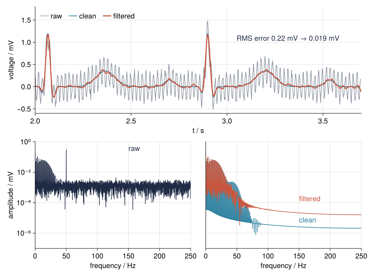
That is the end point. Two filters get there, a 50 Hz notch for the hum and a Butterworth low-pass at 40 Hz for the noise, and each passes over the record once forward and once in reverse. The RMS error shrinks elevenfold, the hum line 560-fold, and every R peak lands within one sample of its true position. The spectra are read as in The Fourier transform in Julia, which mentions getting rid of hum by suppressing the spectrum near 50 Hz and transforming back. A digital filter does that job one sample at a time, and Step 2 explains what this buys you.

Setup

Install the registered packages once with import Pkg; Pkg.add(["DSP", "FFTW", "CairoMakie"]); Random, Statistics, and Printf ship with Julia. The waves table holds the Gaussian bumps of one beat, named P to T as cardiologists name them, each placed relative to the R peak. Heartbeat, hum, and noise live in arrays of their own, which lets Step 5 send each through the filters alone.

using DSP, FFTW, Random, Statistics, Printf, CairoMakie

const fs = 500.0                           # sampling rate, Hz
t = (0:4999) ./ fs                         # 10 s

waves = [                                  # P, Q, R, S, T: offset from the R peak / s, amplitude / mV, width / s
    (offset = -0.20, amp = 0.15, width = 0.025),
    (offset = -0.03, amp = -0.15, width = 0.008),
    (offset = 0.00, amp = 1.20, width = 0.010),
    (offset = 0.03, amp = -0.25, width = 0.008),
    (offset = 0.30, amp = 0.35, width = 0.050),
]
r_times = 0.4:60/72:10                     # 72 beats per minute
ecg = sum(w.amp .* exp.(-0.5 .* ((t .- t_r .- w.offset) ./ w.width) .^ 2)
          for t_r in r_times for w in waves)

hum = 0.30 .* cos.(2π .* 50 .* t .+ 0.7)   # the phase of the mains at the start is arbitrary
noise = 0.05 .* randn(Xoshiro(42), length(t))
x = ecg .+ hum .+ noise                    # what the amplifier delivers, mV

rms(d) = sqrt(mean(abs2, d))

const INK, ACCENT, SECOND, MUTED = "#1f2a44", "#c8553d", "#2a7f9e", "#8a8f98"
set_theme!(Theme(                          # the look of every figure below
    size = (770, 396), fontsize = 17,
    palette = (color = [INK, ACCENT, SECOND, MUTED],),
    Axis = (topspinevisible = false, rightspinevisible = false, xgridvisible = true, ygridvisible = true),
    Lines = (linewidth = 2.5,),
))

@printf("%d samples at %.0f Hz, raw record off by %.2f mV RMS\n", length(t), fs, rms(x .- ecg))

5000 samples at 500 Hz, raw record off by 0.22 mV RMS

Step 1: Look at the spectrum of the raw record

As in the Fourier tutorial, the amplitude spectrum is rfft times 2/N, so a sinusoid of 0.30 mV shows up as a line of 0.30 mV. The axis is logarithmic because the hum towers 250 times over the noise floor. Gains from here on are in decibels, twenty times the base-10 logarithm of an amplitude ratio: a factor of 0.1 is -20 dB, a factor of 0.71 is -3 dB.

Copy

freq = rfftfreq(length(t), fs)
amplitude(s) = 2 .* abs.(rfft(s)) ./ length(s)   # mV

A_raw = amplitude(x)
k50 = argmin(abs.(freq .- 50))
floor_raw = median(A_raw[freq .> 100])
@printf("hum line      %.2f mV at %.1f Hz\n", A_raw[k50], freq[k50])
for n in (5, 20, 34)
    f_n = n * 72 / 60                      # the n-th harmonic of the heart rate
    @printf("harmonic %2d   %.4f mV at %.1f Hz\n", n, A_raw[argmin(abs.(freq .- f_n))], f_n)
end
@printf("noise floor   %.4f mV (median above 100 Hz)\n", floor_raw)

fig = Figure()
ax = Axis(fig[1, 1], xlabel = "frequency / Hz", ylabel = "amplitude / mV", yscale = log10)
lines!(ax, freq, A_raw, color = INK, linewidth = 1.4)
vlines!(ax, 40, color = MUTED, linestyle = :dash, linewidth = 1.4)
text!(ax, 38, 2e-5, text = "40 Hz", color = MUTED, align = (:right, :bottom))
text!(ax, 53, 0.2, text = "hum, 0.30 mV", color = INK)
text!(ax, 3, 0.18, text = "ECG\nharmonics", color = INK)
text!(ax, 150, 0.005, text = "noise floor", color = INK)
limits!(ax, 0, 250, 1e-5, 2)
fig

hum line      0.30 mV at 50.0 Hz
harmonic  5   0.0783 mV at 6.0 Hz
harmonic 20   0.0248 mV at 24.0 Hz
harmonic 34   0.0036 mV at 40.8 Hz
noise floor   0.0012 mV (median above 100 Hz)

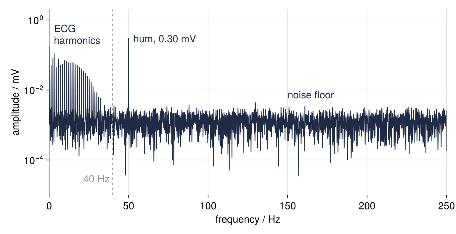
A heart at 72 beats per minute repeats at 1.2 Hz, and anything that repeats at 1.2 Hz has energy only at whole multiples of it: the comb on the left. Its teeth drop from 0.078 mV at 6 Hz to 0.0036 mV at 40.8 Hz, three times the 0.0012 mV floor, and past them only the hum rises out of the noise. So cut above about 40 Hz, and give 50 Hz a filter of its own, since it lies too close for one cut to catch it.

Step 2: Design a notch for the hum and read its response

The Fourier tutorial's repair can only start once the whole record is in. A digital filter looks back instead: each new output is a weighted sum of a few recent inputs and of its own recent outputs, so it works on a record of any length, even one still coming in. DSP.jl holds the weights in a filter object, which filt, filtfilt, and freqresp all accept.

Seen from the spectrum, a filter multiplies each frequency by a complex number, the frequency response, which scales its amplitude and shifts its phase; the gain is its size in dB. freqresp(filter, w) expects w in radians per sample, the angle a frequency advances between two samples (0.63 for 50 Hz at 500 Hz), and the helper gain_dB converts from hertz. A notch's sharpness is its quality factor Q, center frequency over -3 dB width. DSP.jl's iirnotch wants that width in hertz, where SciPy wants Q, so Q = 30 at 50 Hz is written 50 / 30:

Copy

gain_dB(filter, f_hz) = 20 .* log10.(abs.(freqresp(filter, 2π .* f_hz ./ fs)))   # Hz to radians per sample

notch = iirnotch(50, 50 / 30; fs = fs)     # 50 Hz, -3 dB width 50/Q Hz with Q = 30

f_check = [45, 49, 50, 51, 55]
for (f_c, g) in zip(f_check, gain_dB(notch, f_check))
    @printf("%3d Hz  %8.2f dB\n", f_c, g)
end

f_grid = range(0, fs / 2, length = 8192)
gain = gain_dB(notch, f_grid)
stop = f_grid[gain .< -3]
@printf("-3 dB band  %.1f to %.1f Hz\n", first(stop), last(stop))

fig = Figure()
ax = Axis(fig[1, 1], xlabel = "frequency / Hz", ylabel = "gain / dB")
lines!(ax, f_grid, gain, color = ACCENT)
hlines!(ax, -3, color = MUTED, linestyle = :dash, linewidth = 1.4)
text!(ax, 31, -6.5, text = "−3 dB", color = MUTED)
text!(ax, 52, -20, text = @sprintf("below −3 dB\n%.1f to %.1f Hz", first(stop), last(stop)), color = ACCENT)
limits!(ax, 30, 70, -40, 3)
fig

 45 Hz     -0.11 dB
 49 Hz     -2.26 dB
 50 Hz   -273.01 dB
 51 Hz     -2.32 dB
 55 Hz     -0.13 dB
-3 dB band  49.2 to 50.8 Hz

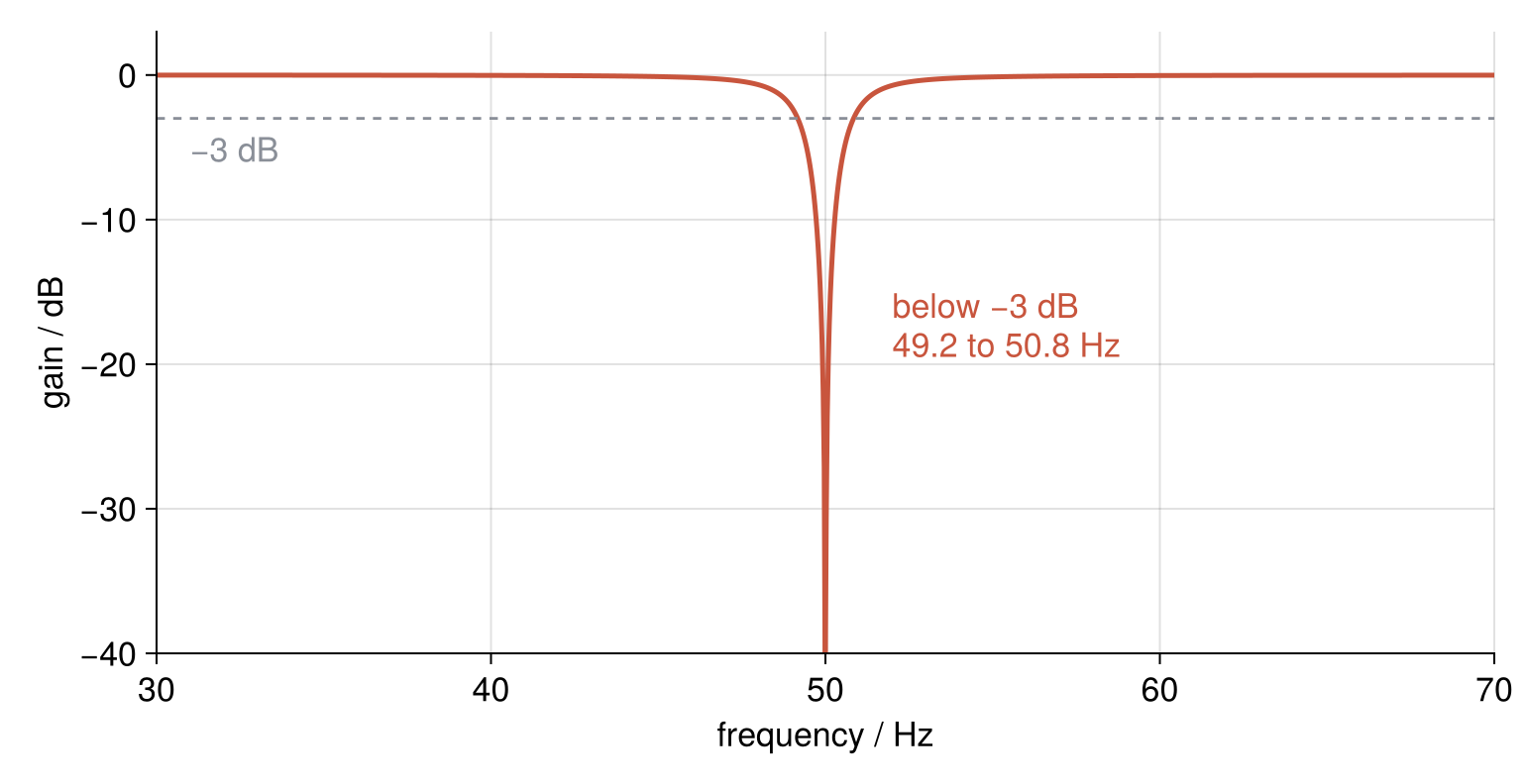
On a grid of 0.03 Hz the dip crosses -3 dB at 49.2 and 50.8 Hz, the 1.7 Hz that 50/30 promised, and 5 Hz to either side the loss is at most 0.13 dB. At 50 Hz itself the gain is below -250 dB, which is rounding error: nothing gets through. A higher Q would spare more heartbeat near 50 Hz, at a price the third pitfall shows.

Step 3: Design a Butterworth low-pass and choose its order

The passband is everything under the cutoff frequency, and a low-pass lets it through while it attenuates the rest. Of all designs, Butterworth's gain is the flattest across the passband, and the name promises nothing else. The order is how many past outputs feed Step 2's weighted sum (textbooks count poles), and each extra one makes the gain drop faster past the cutoff. digitalfilter(Lowpass(40), Butterworth(N); fs = fs) hands back a filter object whose weights you never touch, evaluated as a cascade of two-pole stages that keeps high orders accurate. Orders 2, 4, and 8 at the same cutoff:

Copy

f_check = [20, 30, 40, 50, 100]
println("order", join(@sprintf("%8d Hz", f_c) for f_c in f_check))

fig = Figure()
ax = Axis(fig[1, 1], xlabel = "frequency / Hz", ylabel = "gain / dB")
for (N, alpha) in [(2, 0.35), (4, 0.65), (8, 1.0)]
    butter = digitalfilter(Lowpass(40), Butterworth(N); fs = fs)
    println(@sprintf("%5d", N), join(@sprintf("%8.1f dB", g) for g in gain_dB(butter, f_check)))
    g = gain_dB(butter, f_grid)
    k = argmin(abs.(f_grid .- 103))        # label each line just above it at 103 Hz
    lines!(ax, f_grid, g, color = (ACCENT, alpha))
    text!(ax, 103, g[k] + 2, text = "order $N", color = ACCENT)
end
vlines!(ax, [40, 50], color = MUTED, linestyle = :dash, linewidth = 1.4)
g8_hum = only(gain_dB(digitalfilter(Lowpass(40), Butterworth(8); fs = fs), [50]))
scatter!(ax, 50, g8_hum, color = ACCENT, markersize = 11)   # where the hum meets order 8
text!(ax, 39, -75, text = "cutoff", color = MUTED, align = (:right, :bottom))
text!(ax, 51, -75, text = replace(@sprintf("hum: order 8 only %.1f dB", g8_hum), "-" => "−"), color = MUTED)
limits!(ax, 0, 150, -80, 3)

lowpass = digitalfilter(Lowpass(40), Butterworth(4); fs = fs)   # the choice
fig

order      20 Hz      30 Hz      40 Hz      50 Hz     100 Hz
    2    -0.2 dB    -1.2 dB    -3.0 dB    -5.5 dB   -18.1 dB
    4    -0.0 dB    -0.4 dB    -3.0 dB    -8.8 dB   -36.1 dB
    8    -0.0 dB    -0.0 dB    -3.0 dB   -16.5 dB   -72.3 dB

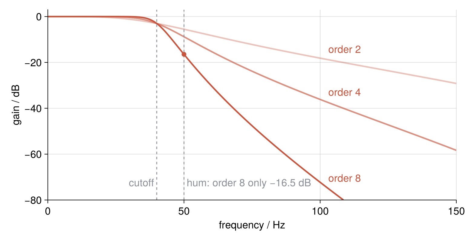
Every order passes 40 Hz at -3 dB, which defines the cutoff. At 100 Hz they read -18, -36, and -72 dB: double the order, double the attenuation. The rule of thumb is 6 dB per order for each octave, a doubling of frequency, above the cutoff. From 40 to 100 Hz is 1.3 octaves, so order 4 should give about -32 dB, and a digital filter beats that because its gain reaches zero at 250 Hz, the Nyquist frequency. At 50 Hz even order 8 only reaches -16.5 dB, so the hum keeps its notch. I take order 4, and the first pitfall shows the price of more.

Step 4: Apply it forward and backward with filtfilt

Both our filters are causal, using only the present sample and the past, and since they feed back their outputs they delay each frequency by its own amount, the group delay. A common delay would leave the beat intact, merely late, and the heart rate unchanged. One that differs between frequencies changes the beat's shape: phase distortion.

filt(f, x) makes one pass from first sample to last, as a bedside monitor must. filtfilt(f, x) filters, reverses, filters again, and reverses back. A comprehension over local maxima above 0.8 mV stands in for DSP.jl's missing peak finder:

Copy

rpeaks(y) = [k for k in 2:length(y)-1 if y[k] > 0.8 && y[k] > y[k-1] && y[k] >= y[k+1]]

y_causal = filt(lowpass, filt(notch, x))
y = filtfilt(lowpass, filtfilt(notch, x))

r_true = rpeaks(ecg)
outputs = [("filt + filt", y_causal), ("filtfilt + filtfilt", y)]
shift = Dict{String,Float64}()
for (name, out) in outputs
    r_out = rpeaks(out)
    @assert length(r_out) == length(r_true) == 12
    shift[name] = mean(r_out .- r_true) / fs * 1000           # ms
    @printf("%-20s R peaks shifted by %+5.1f ms, RMS error %.3f mV\n", name, shift[name], rms(out .- ecg))
end

beat = 1.80 .< t .< 2.45
fig = Figure(size = (770, 484))
axs = [Axis(fig[i, 1], ylabel = "voltage / mV") for i in 1:2]
linkxaxes!(axs...)
hidexdecorations!(axs[1], grid = false)
axs[2].xlabel = "t / s"
for (ax, (name, out)) in zip(axs, outputs)
    lines!(ax, t[beat], ecg[beat], color = SECOND, linewidth = 1.7)
    lines!(ax, t[beat], out[beat], color = ACCENT)
    vlines!(ax, r_times[3], color = MUTED, linestyle = :dash, linewidth = 1.4)
    text!(ax, 2.11, 0.9, text = "$name: R peak $(round(Int, shift[name])) ms late", color = ACCENT)
    ylims!(ax, -0.36, 1.3)
end
text!(axs[1], 1.82, 0.45, text = "clean ECG", color = SECOND)
text!(axs[1], r_times[3] - 0.004, -0.33, text = "true R time", color = MUTED, align = (:right, :bottom))
xlims!(axs[2], 1.80, 2.45)
fig

filt + filt          R peaks shifted by +11.2 ms, RMS error 0.142 mV
filtfilt + filtfilt  R peaks shifted by  -0.2 ms, RMS error 0.019 mV

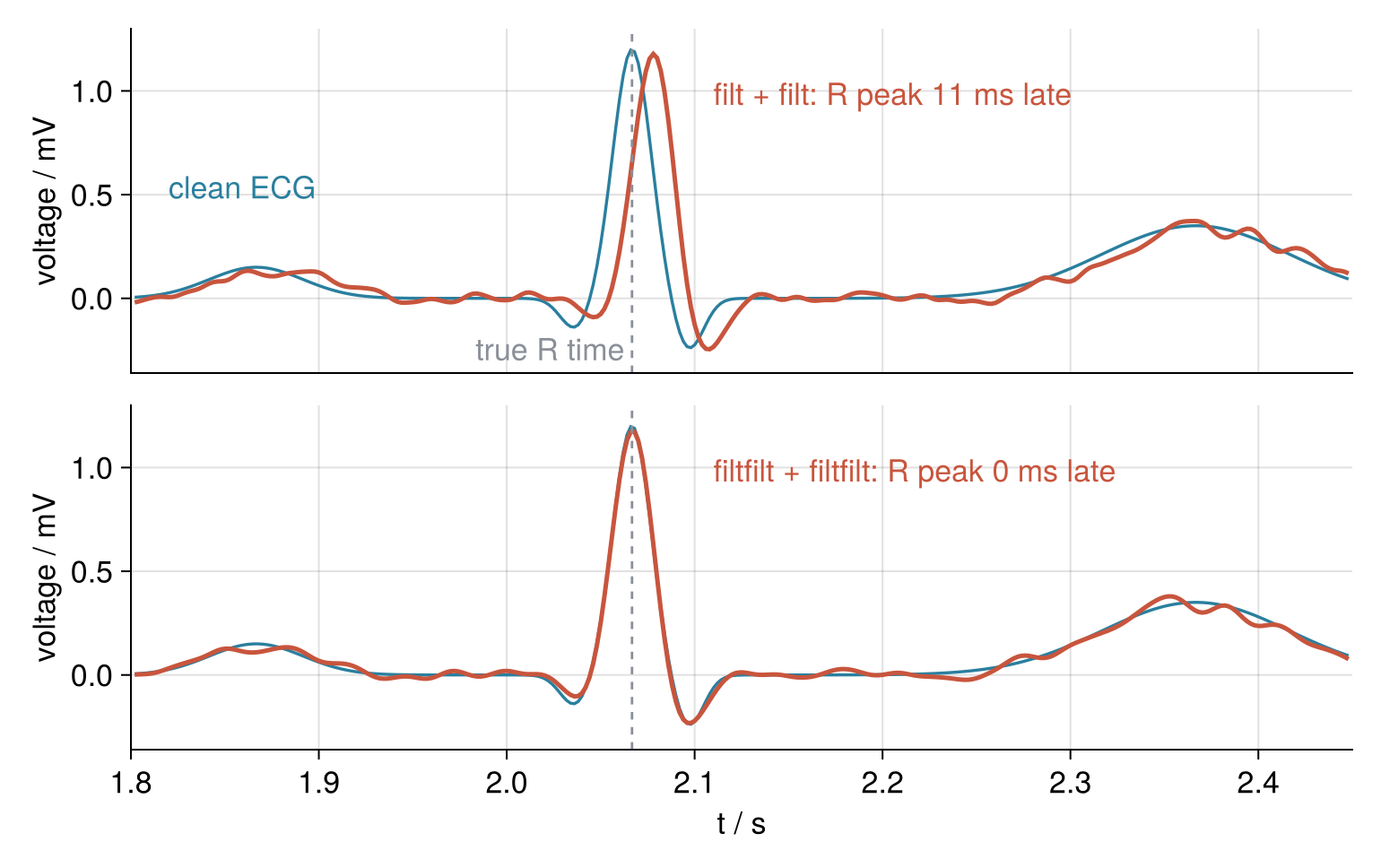
With filt the R peaks come 11.2 ms late, most of the 0.142 mV error. With filtfilt eleven of twelve peaks sit on their true sample, one a sample early from the noise, and the error falls to 0.019 mV. The reversed pass undoes the forward delay: the pair is zero-phase. grpdelay shows how unequal the causal delay is. Sliding the causal heartbeat back by its common delay leaves only the shape change:

w_probe = 2π .* [1.2, 10, 30] ./ fs                    # Hz to radians per sample
tau = (grpdelay(notch, w_probe) .+ grpdelay(lowpass, w_probe)) ./ fs .* 1000   # delays of a chain add; ms
@printf("group delay of filt + filt: %.1f ms at 1.2 Hz, %.1f ms at 10 Hz, %.1f ms at 30 Hz\n", tau...)

ecg_causal = filt(lowpass, filt(notch, ecg))
ecg_left = filtfilt(lowpass, filtfilt(notch, ecg))
advance(s, d) = irfft(rfft(s) .* cis.(2π .* freq .* d ./ fs), length(s))   # earlier by d samples, d need not be whole
inner = 251:4750                                       # skip 0.5 s at each end, where the advance wraps around
d_best = argmin(d -> rms((advance(ecg_causal, d) .- ecg)[inner]), 0:0.01:10)
@printf("ECG alone, off from the truth: filt advanced %.2f samples %.4f mV, filtfilt %.4f mV\n",
        d_best, rms((advance(ecg_causal, d_best) .- ecg)[inner]), rms((ecg_left .- ecg)[inner]))

group delay of filt + filt: 10.3 ms at 1.2 Hz, 10.6 ms at 10 Hz, 15.1 ms at 30 Hz
ECG alone, off from the truth: filt advanced 5.34 samples 0.0050 mV, filtfilt 0.0036 mV

The delay grows by 5 ms from the 1.2 Hz heart rate to 30 Hz, about the highest frequency in the QRS complex, the sharp Q, R, and S bumps. At its best shift, 5.34 samples, the causal heartbeat is off by 0.0050 mV, 1.4 times what filtfilt leaves. On this beat the shape barely suffers; the 11 ms delay is the damage.

The gain counts twice, so the pair is at -6 dB at 40 Hz. Its -3 dB point is where the squared response drops under 0.71:

f_3dB(filter) = f_grid[findfirst(abs2.(freqresp(filter, 2π .* f_grid ./ fs)) .< 10^(-3 / 20))]  # squared: applied twice
@printf("-3 dB point under filtfilt: designed at 40 Hz %.1f Hz, designed at 45 Hz %.1f Hz\n",
        f_3dB(lowpass), f_3dB(digitalfilter(Lowpass(45), Butterworth(4); fs = fs)))

-3 dB point under filtfilt: designed at 40 Hz 36.0 Hz, designed at 45 Hz 40.5 Hz

Under filtfilt the 40 Hz design is down 3 dB at 36 Hz, and a 45 Hz design puts that point at 40.5 Hz. I keep 40 Hz, since Step 1's comb had sunk to three times the floor by 40.8 Hz.

Step 5: Check in the spectrum what went and what stayed

The first three lines need only your recording, the last two the truth:

A_y, A_ecg = amplitude(y), amplitude(ecg)
floor_y = median(A_y[freq .> 100])
comb = [argmin(abs.(freq .- n * 1.2)) for n in 1:20]   # the heartbeat's lines up to 24 Hz
kept = 100 .* A_y[comb] ./ A_raw[comb]
@printf("50 Hz line          %.2f mV -> %.4f mV\n", A_raw[k50], A_y[k50])
@printf("floor above 100 Hz  %.4f mV -> %.6f mV, %.0f dB\n", floor_raw, floor_y, 20 * log10(floor_y / floor_raw))
@printf("comb up to 24 Hz    %.1f to %.1f %% of the raw lines\n", minimum(kept), maximum(kept))
@printf("RMS error           %.2f mV -> %.3f mV\n", rms(x .- ecg), rms(y .- ecg))
@printf("R peak height       %.0f %% of the truth\n", 100 * mean(y[r_true] ./ ecg[r_true]))

50 Hz line          0.30 mV -> 0.0005 mV
floor above 100 Hz  0.0012 mV -> 0.000019 mV, -36 dB
comb up to 24 Hz    98.5 to 100.0 % of the raw lines
RMS error           0.22 mV -> 0.019 mV
R peak height       98 % of the truth

The hum line shrank 560-fold and the comb up to 24 Hz kept 98.5 to 100 % of its raw height. The R peaks keep 98 % of theirs.

The floor above 100 Hz fell 36 dB, though the pair takes 72 dB there (Step 3's 36 dB, twice). The transform assumes the record repeats, so it sees a jump from the last sample back to the first, and a jump needs every frequency to build it, at slowly falling amplitudes: spectral leakage. A straight line from 0 to the jump's height has that jump and nothing else, so its spectrum is the jump's share of the floor. The loop filters the parts one at a time to find where the jump comes from, which works because the filters are linear:

jump = y[end] - y[1]
ramp = jump .* t ./ t[end]
@printf("jump from last to first sample %+.3f mV; ramp floor %.6f mV\n", jump, median(amplitude(ramp)[freq .> 100]))
for (name, part) in [("ECG", ecg), ("hum", hum), ("noise", noise)]
    part_out = filtfilt(lowpass, filtfilt(notch, part))
    @printf("  share from the %-5s %+.3f mV\n", name, part_out[end] - part_out[1])
end

jump from last to first sample -0.057 mV; ramp floor 0.000013 mV
  share from the ECG   +0.012 mV
  share from the hum   -0.093 mV
  share from the noise +0.023 mV

The ramp makes two thirds of the floor: above 40 Hz the filters did their job, and most of the jump is hum the notch left at the edges (the third pitfall).

The 0.019 mV left is predictable. Noise from randn is white, its power spread evenly from 0 to 250 Hz. A 40 Hz low-pass leaves 40/250 of it, and RMS goes as the square root, so 0.05 mV × √(40/250) should survive:

predicted = 0.05 * sqrt(40 / (fs / 2))
noise_left = filtfilt(lowpass, filtfilt(notch, noise))
@printf("in-band noise: predicted %.4f mV, noise filtered alone %.4f mV\n", predicted, rms(noise_left))

in-band noise: predicted 0.0200 mV, noise filtered alone 0.0189 mV

The measurement is 6 % lower, since the pair is 6 dB down at 40 Hz.

Copy

fig = Figure(size = (880, 660))
ax_t = Axis(fig[1, 1:2], xlabel = "t / s", ylabel = "voltage / mV")
two = 2.0 .< t .< 3.7
lines!(ax_t, t[two], x[two], color = (INK, 0.5), linewidth = 1.4, label = "raw")
lines!(ax_t, t[two], ecg[two], color = SECOND, linewidth = 1.7, label = "clean")
lines!(ax_t, t[two], y[two], color = ACCENT, label = "filtered")
text!(ax_t, 3.05, 1.0, text = @sprintf("RMS error %.2f mV → %.3f mV", rms(x .- ecg), rms(y .- ecg)), color = INK)
limits!(ax_t, 2.0, 3.7, -0.6, 1.8)
axislegend(ax_t, position = :lt, orientation = :horizontal, framevisible = false)

ax_b = Axis(fig[2, 1], xlabel = "frequency / Hz", ylabel = "amplitude / mV", yscale = log10)
ax_a = Axis(fig[2, 2], xlabel = "frequency / Hz", yscale = log10)
linkyaxes!(ax_b, ax_a)
lines!(ax_b, freq, A_raw, color = INK, linewidth = 1.4)
text!(ax_b, 150, 0.2, text = "raw", color = INK)
lines!(ax_a, freq, A_ecg, color = SECOND, linewidth = 1.4)
lines!(ax_a, freq, A_y, color = ACCENT, linewidth = 1.4)
text!(ax_a, 150, 1e-4, text = "filtered", color = ACCENT)
text!(ax_a, 150, 4e-6, text = "clean", color = SECOND)
for ax in (ax_b, ax_a)
    limits!(ax, 0, 250, 1e-7, 1)
    ax.yticks = ([1e-6, 1e-4, 1e-2, 1], ["10⁻⁶", "10⁻⁴", "10⁻²", "10⁰"])   # every other decade, as in Step 1
end
hideydecorations!(ax_a, grid = false)      # the linked axis would repeat the left one's labels
colgap!(fig.layout, 1, 36)                 # keeps "250" and "0" of the two x axes apart
fig

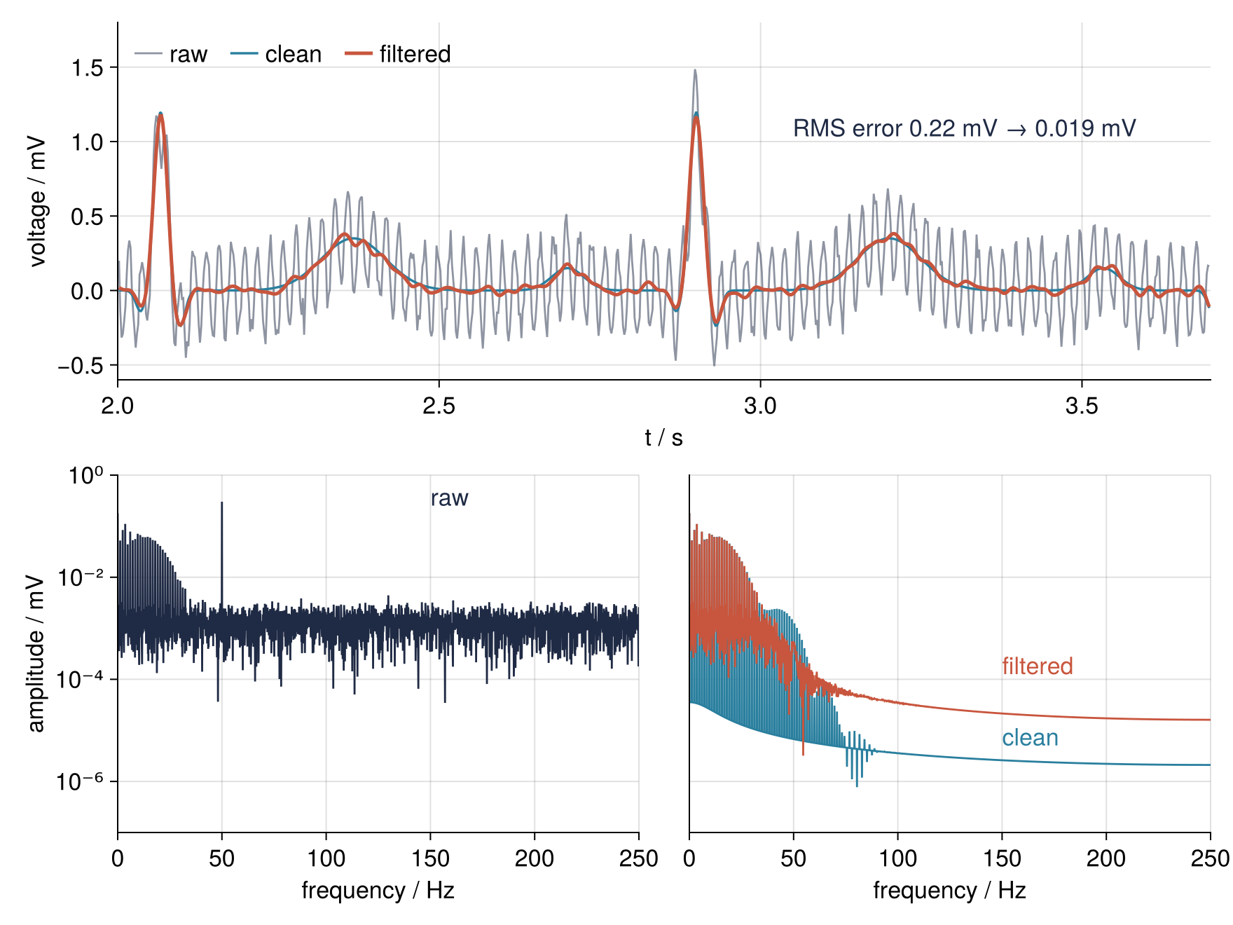
Under 30 Hz the filtered spectrum traces the clean one, and past about 90 Hz both show the smooth spectrum of a jump, as the clean record, too, ends away from where it begins. What remains is noise in the heartbeat's own band, beyond any filter's reach, and the square-root rule predicts it only for white noise: noise that grows toward low frequencies leaves more.

Pitfalls

Turning up the order until it rings. Every QRS complex grows small false wiggles in front of it and behind it. Hit a filter with one brief kick and it answers with an oscillation that dies away slowly, its impulse response. A steep cutoff makes that oscillation long and large, and each sharp edge in the signal sets it going. A step from 0 to 1 through the zero-phase low-pass measures it:

edge = [zeros(500); ones(500)]
for N in (2, 4, 8)
    s = filtfilt(digitalfilter(Lowpass(40), Butterworth(N); fs = fs), edge)
    @printf("order %d: overshoot %.1f %%, undershoot %.1f %%\n", N, 100 * (maximum(s) - 1), -100 * minimum(s[1:500]))
end

order 2: overshoot 3.6 %, undershoot 3.6 %
order 4: overshoot 6.9 %, undershoot 6.9 %
order 8: overshoot 8.4 %, undershoot 8.4 %

Order 2 overshoots by 3.6 %, order 8 by 8.4 %, and the undershoot before the edge matches the overshoot after it, because the reversed pass mirrors the ringing in time. Pick the smallest order that Step 3's table shows is enough, never a larger one.

Forgetting fs, and the normalized frequency. Without fs, DSP.jl counts frequency in half-cycles per sample, so 1.0 is the Nyquist frequency, fs / 2. Lowpass(40) then asks for a cutoff forty times above it and fails, and the usual repair, Lowpass(40 / fs), runs without complaint:

try
    digitalfilter(Lowpass(40), Butterworth(4))
catch err
    println(sprint(showerror, err))
end
wrong = digitalfilter(Lowpass(40 / fs), Butterworth(4))
@printf("Lowpass(40 / fs) without fs is -3 dB at %.1f Hz\n", f_grid[findfirst(gain_dB(wrong, f_grid) .< -3)])

DomainError with 40.0:
frequencies must be less than the Nyquist frequency 1.0
Lowpass(40 / fs) without fs is -3 dB at 20.0 Hz

You get 20 Hz instead of 40, without a warning. Pass fs = fs to every digitalfilter and iirnotch. freqresp takes no fs at all, so convert hertz to radians per sample there yourself, as gain_dB does.

Trusting the first and last half second. The middle of the filtered record is free of hum, yet near either end the 50 Hz wobble is back. Filter the hum by itself to see how much:

hum_left = filtfilt(notch, hum)
n01, n05 = round(Int, 0.1fs), round(Int, 0.5fs)
@printf("first 0.1 s            %.3f mV\n", maximum(abs, hum_left[1:n01]))
@printf("0.5 s from either end  %.4f mV\n", maximum(abs, hum_left[n05+1:end-n05]))
@printf("between 4 and 6 s      %.0e mV\n", maximum(abs, hum_left[4 .< t .< 6]))

first 0.1 s            0.143 mV
0.5 s from either end  0.0105 mV
between 4 and 6 s      1e-10 mV

Half of the 0.30 mV survives in the first 0.1 s, a billionth of it between 4 and 6 s. A notch has to watch the hum for a while before it cancels it, and the narrower the notch, the longer it takes: the settling time is roughly one over π times the width, 1/(π · 1.67 Hz) = 0.19 s. The padding filtfilt adds is three samples per pole, so 6 samples or 12 ms for the two-pole notch. It is the edge of the record flipped upside down and mirrored, which is not a continuation of the hum, so the settling happens inside your record. DSP.jl's filtfilt offers no longer or different padding. Record a little more than you need and cut 0.5 s from each end, which brings the residue down to 0.011 mV, or lower Q when the edges matter.

Variations

• Baseline wander. A breathing patient and shifting electrodes make the baseline drift at under 0.5 Hz. Swap the low-pass for digitalfilter(Bandpass(0.5, 40), Butterworth(2); fs = fs), which removes the drift as well.
• 60 Hz and its harmonics. Mains in North America run at 60 Hz, and nonlinear loads on the grid add odd harmonics at 180 and 300 Hz. DSP.jl has no comb notch, so use one iirnotch per line: filter with each in turn, or multiply them, iirnotch(60, 2; fs = fs) * iirnotch(180, 6; fs = fs), into a single filter that applies both.
• Filtering as the data arrives. state = DF2TFilter(lowpass), a filter in the structure textbooks call direct form II transposed, keeps its memory between calls, so each filt(state, chunk) picks up where the last chunk ended. The 11 ms delay of Step 4 comes with it.
• A strain gauge instead of a heart. A strain-gauge bridge read at 1 kHz, its signal under 20 Hz, picks up the same hum and noise. Set fs = 1000, a cutoff near 20 Hz, and the notch at your mains frequency, and keep the rest of the chain.

Cheat sheet

notch = iirnotch(f0, f0 / Q; fs = fs)                          # second argument: -3 dB width in Hz, not Q
lowpass = digitalfilter(Lowpass(fc), Butterworth(N); fs = fs)  # always fs = fs
gain = 20 .* log10.(abs.(freqresp(lowpass, 2π .* f ./ fs)))    # f in Hz to radians per sample; no fs here
y = filtfilt(lowpass, filtfilt(notch, x))                      # zero phase; gain applied twice, -6 dB at fc
y = filt(lowpass, filt(notch, x))                              # causal, starts from rest; delayed
state = DF2TFilter(lowpass); filt(state, chunk)                # keeps its memory from chunk to chunk
σ * sqrt(fc / (fs / 2))                                        # noise left in 0 to fc, white noise only
n = round(Int, 0.5fs); y = y[n+1:end-n]                        # drop the edges where the notch settles

Further reading

• The DSP.jl documentation on filter design and filtering, with digitalfilter, iirnotch, filt, filtfilt, and freqresp, and the package home.
• For the filter chapters, Steven W. Smith's The Scientist and Engineer's Guide to Digital Signal Processing; for the mathematics underneath, Oppenheim and Schafer, Discrete-Time Signal Processing.
• Related tutorials on this site: The Fourier transform in Julia: asking a signal how much of each frequency it contains, and Filtering with scipy.signal: mains hum and noise out of an ECG, the same tutorial in Python.
• Download the notebook. It was executed with the library versions in the header.