The Fourier transform in Julia: asking a signal how much of each frequency it contains

The question

Here is the kind of record the Fourier transform was made for: a month of sea level at a harbor, read once an hour, 720 readings in all.

Show code

using CairoMakie, Random, Statistics, Printf

const INK, ACCENT, SECOND, MUTED = "#1f2a44", "#c8553d", "#2a7f9e", "#8a8f98"
set_theme!(Theme(
    size = (770, 396), fontsize = 17,
    palette = (color = [INK, ACCENT, SECOND, MUTED],),
    Axis = (topspinevisible = false, rightspinevisible = false, xgridvisible = true, ygridvisible = true),
    Lines = (linewidth = 2.5,),
))

# Not a real gauge: four tidal constituents plus noise, so that the answer
# can be graded at the end. Pretend you never opened this cell.
t = range(0, step = 1.0, length = 30 * 24)          # hours
constituents = [                                    # period / h, amplitude / m, phase
    (name = "M2", P = 12.4206, A = 1.00, φ = 0.0),
    (name = "S2", P = 12.0000, A = 0.45, φ = 0.7),
    (name = "K1", P = 23.9345, A = 0.30, φ = π / 2),
    (name = "O1", P = 25.8193, A = 0.20, φ = 1.2),
]
h = sum(c.A .* cos.(2π .* t ./ c.P .+ c.φ) for c in constituents)
h .+= 0.15 .* randn(Xoshiro(42), length(t))         # weather and the gauge itself

fig = Figure(size = (880, 330))
ax = Axis(fig[1, 1], xlabel = "time / days", ylabel = "sea level / m")
lines!(ax, t ./ 24, h, color = INK, linewidth = 1.4)
xlims!(ax, 0, 30)
fig

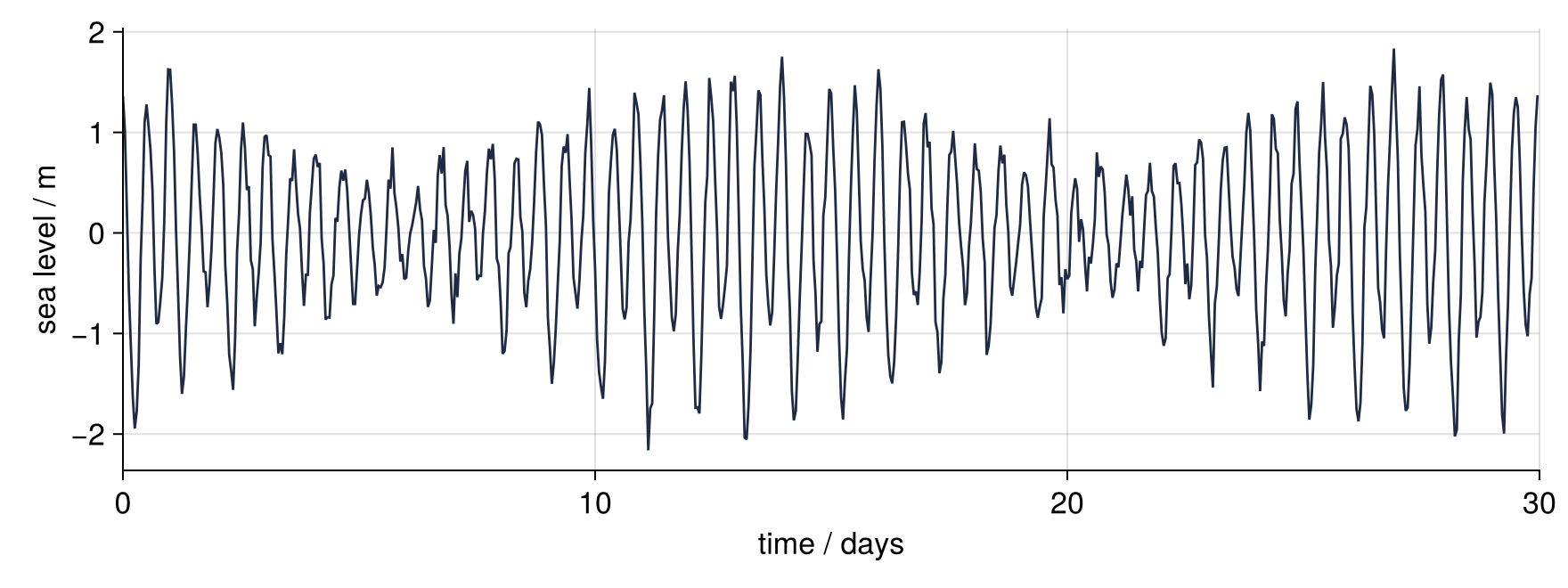
Two features stand out at once. The water rises and falls roughly twice a day, and the size of those swings breathes: about a week of big ones, a week of small ones, then big again. Anyone who has tied up a boat knows both, as the tide itself and as the alternation of spring and neap tides every two weeks.

What the eye cannot read off is how many separate rhythms make up this curve, what each period is to three decimals, and how much each one contributes. A harbor that prints next year's tide tables needs exactly those numbers, and the curve above hides them. The twice-daily rise is in fact two rhythms, one of 12.42 h set by the Moon and one of 12.00 h set by the Sun, and the fortnightly breathing is the beat between them. Splitting a record into its rhythms is the job of the Fourier transform. The pages below are about how it does that job; the library call, rfft from FFTW.jl, waits until the end and takes a handful of lines.

The idea: compare the signal with a probe

Say you want to know whether the record holds an oscillation with a 12 h period. Make one yourself, \(\cos(2\pi f t)\) with \(f = 1/12\) cycles per hour, and call it the probe. Multiply record and probe reading by reading, then average the products.

When the rhythm is in the record, water and probe climb and sink together, so the product stays mostly above zero and its average is clearly positive. When the rhythm is absent, the probe is in step with the water part of the time and against it the rest, positive and negative products cancel, and the average lands near zero. In Julia the whole test is one line. The factor 2 makes the result read as an amplitude in meters, and the Formalization shows where it comes from.

Here are three probes, one at 0.0700, one at the lunar 0.0805 (the 12.42 h period), and one at 0.0900 cycles per hour. The panels draw only the first 72 h, picked by the mask t .< 72, so that the shaded product stays readable. The average printed in each panel is still taken over all 30 days. Over three days alone the products have had no time to cancel, and the numbers would come out different.

"""Twice the mean of record times cosine probe: the amplitude, in m, of frequency f."""
probe_average(f) = 2 * mean(h .* cos.(2π * f .* t))

window = t .< 72
fig = Figure(size = (880, 715))
panels = [Axis(fig[i, 1], ylabel = "m") for i in 1:3]
for (ax, f) in zip(panels, [0.0700, 1 / 12.4206, 0.0900])
    probe = cos.(2π * f .* t)
    lines!(ax, t[window], h[window], color = INK, label = "signal")
    lines!(ax, t[window], probe[window], color = SECOND, linewidth = 1.2, label = "probe")
    band!(ax, t[window], zeros(count(window)), (h .* probe)[window],
          color = (ACCENT, 0.35), label = "product")
    text!(ax, 0.99, 0.95, space = :relative, align = (:right, :top),
          text = @sprintf("f = %.4f /h   30-day average = %+.2f m", f, probe_average(f)))
    xlims!(ax, 0, 72); ylims!(ax, -2.6, 3.4)
    ax.xticks = 0:24:72
end
linkxaxes!(panels...)
hidexdecorations!.(panels[1:2], grid = false)
panels[3].xlabel = "time / h"
axislegend(panels[1], position = :lt, orientation = :horizontal, framevisible = false)
fig

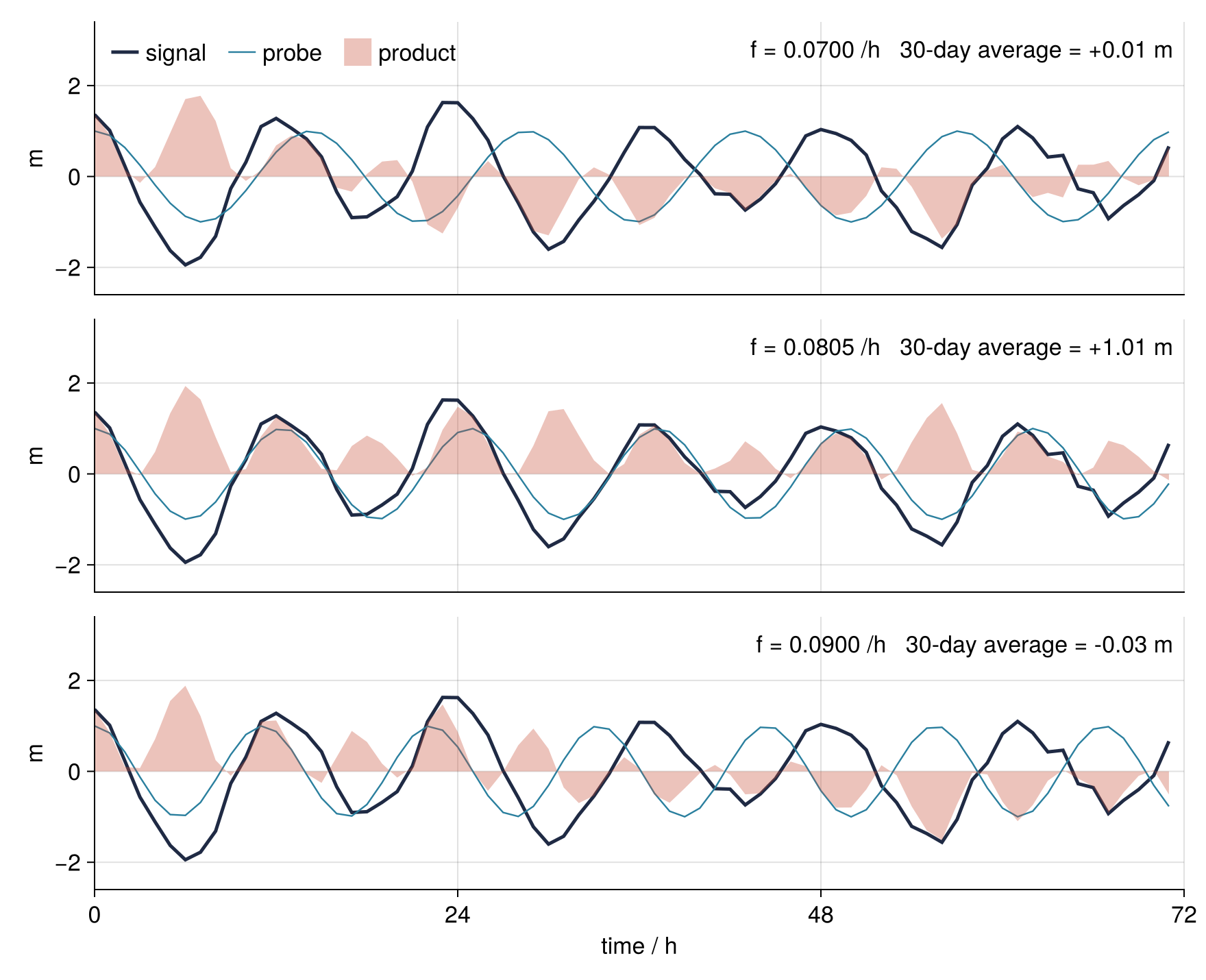
At 0.0700 cycles per hour the shaded product flips sign every few hours, and the 30-day average is +0.01 m, which is nothing. At the lunar frequency the product sits above zero almost everywhere and averages +1.01 m, the amplitude M2 was built with, give or take the noise. At 0.0900 it is down to −0.03 m. One multiplication and one mean have found a rhythm and measured it.

Now let the probe frequency slide and keep track of the average as it goes. The curve that comes out is a spectrum, and the animation draws it one probe at a time:

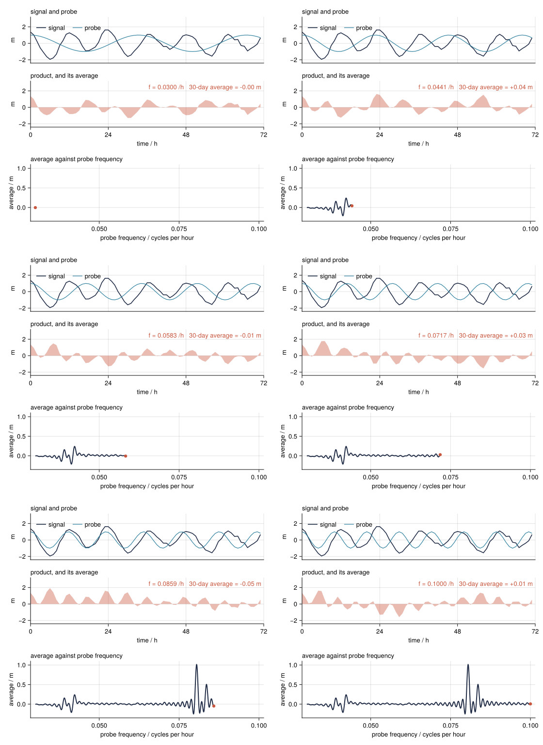
The probe frequency sweeps from 0.03 to 0.10 cycles per hour. Top: the first three days of the record and the probe. Middle: their product over those three days; its average over all 30 days is the number printed and plotted below. Bottom: the average against probe frequency, which jumps up where the probe matches a tide.

How I built this: Visualization tutorial "Animating a probe sweep", planned.

The same sweep over 2,000 frequencies, where the dot in probe_average.(f) calls the function once for every frequency in the range:

f = range(0.01, 0.12, length = 2000)
cos_sweep = probe_average.(f)

fig = Figure(size = (880, 352))
ax = Axis(fig[1, 1], xlabel = "probe frequency / cycles per hour", ylabel = "average / m")
lines!(ax, f, cos_sweep, color = INK)
xlims!(ax, 0.01, 0.12)
fig

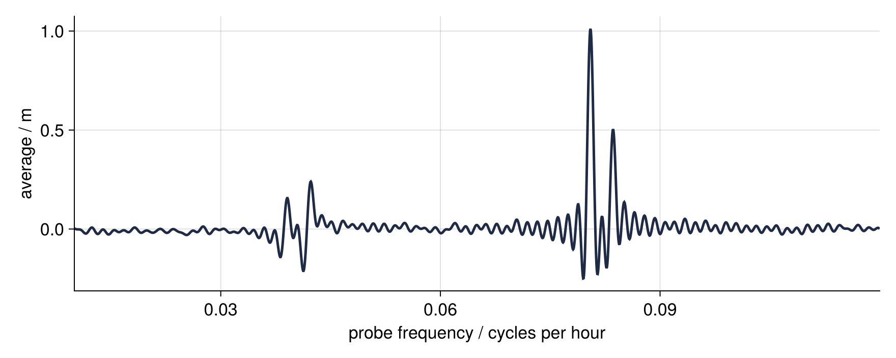
Peaks stand near 0.0805 and 0.0833 cycles per hour, which are 12.42 h and 12.00 h, and near 0.04 there is a small up-and-down twitch. Something is missing. The record clearly swings once a day as well, and this curve has no peak for it.

The lost phase, and why the transform is complex

A cosine probe is blind to a rhythm that runs a quarter period ahead of it. Against such a sine, the product is positive for a quarter cycle and negative for the next, and the average vanishes up to the noise. K1 in this record has exactly that phase, π/2, so the cosine probe registers it only as the twitch near 0.04, an up and a down that cross zero where the peak belongs. O1, with a phase of 1.2, comes through at a fraction of its size.

So send two probes, a cosine and a sine at the same frequency, and keep both averages. For a rhythm \(A\cos(2\pi f t + \varphi)\) the cosine probe collects \((A/2)\cos\varphi\) and the sine probe \(-(A/2)\sin\varphi\) (the Formalization shows why). Flip the sign of the second and the two are the legs of a right triangle whose hypotenuse is \(A/2\) for every \(\varphi\). Euler's formula,

\[e^{-2\pi i f t} = \cos(2\pi f t) - i\sin(2\pi f t),\]

lets both probes travel as one complex number, with the cosine average as its real part and the sine average, sign flipped by the minus in front of \(i\), as its imaginary part. The modulus is then half the amplitude whatever the phase, and the argument is the phase. The complex numbers in a Fourier transform are bookkeeping for a pair of probes and nothing more. In Julia the imaginary unit is im:

spectrum(f) = 2 * abs(mean(h .* exp.(-2π * im * f .* t)))
amp = spectrum.(f)

fig = Figure(size = (880, 352))
ax = Axis(fig[1, 1], xlabel = "probe frequency / cycles per hour", ylabel = "amplitude / m")
lines!(ax, f, amp, color = INK)
for c in constituents
    peak = maximum(amp[abs.(f .- 1 / c.P) .< 0.001])
    text!(ax, 1 / c.P, peak, text = c.name, color = ACCENT, align = (:center, :bottom), offset = (0, 6))
    @printf("%s   built with %.2f m   read back %.2f m\n", c.name, c.A, peak)
end
xlims!(ax, 0.01, 0.12); ylims!(ax, 0, 1.15)
fig

M2   built with 1.00 m   read back 1.01 m
S2   built with 0.45 m   read back 0.50 m
K1   built with 0.30 m   read back 0.31 m
O1   built with 0.20 m   read back 0.21 m

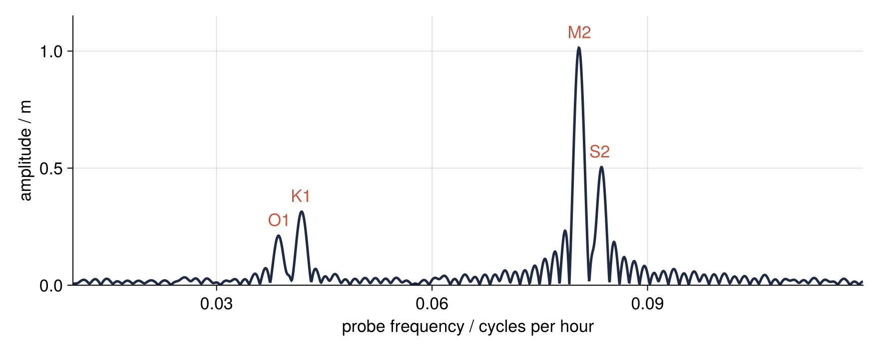
Four peaks now, two near half a day and two near a whole day. Oceanographers call these constituents M2 and S2, the principal lunar and solar semidiurnal tides, and K1 and O1, two of the diurnal ones. The record was assembled from exactly these four, and the spectrum hands them back at 1.01, 0.50, 0.31 and 0.21 m against the 1.00, 0.45, 0.30 and 0.20 m that went in, K1 included. S2 reads 0.05 m high because it stands on the flank of the much taller M2 peak. Why a peak has flanks at all is the business of the next section.

Formalization

Up to a normalization, the average of signal times complex probe is the Fourier transform. For a signal \(x(t)\) it reads

\[X(f) = \int_{-\infty}^{\infty} x(t)\, e^{-2\pi i f t}\, dt .\]

The modulus \(|X(f)|\) says how strongly frequency \(f\) is present and the argument \(\arg X(f)\) gives its phase. Run backwards, \(x(t) = \int X(f)\, e^{+2\pi i f t}\, df\) rebuilds the signal from its frequencies: any reasonable signal is a sum of oscillations, and \(X\) lists the ingredients.

A gauge does not deliver \(x(t)\) but \(N\) readings \(x_n\) at spacing \(\Delta t\), and the integral turns into a sum,

\[X_k = \sum_{n=0}^{N-1} x_n\, e^{-2\pi i k n / N}, \qquad f_k = \frac{k}{N \Delta t}, \qquad k = 0, 1, \dots, N-1,\]

the discrete Fourier transform. A cosine of amplitude \(A\) contributes \(|X_k| = NA/2\) at its own frequency, so \(2|X_k|/N\) reads in meters, and that is the 2 in probe_average. It comes from a product rule for cosines: two cosines multiplied give half a cosine at the difference of their frequencies plus half a cosine at the sum. The sum term always oscillates and averages out. The difference term does too, unless the two frequencies match, and then it is the constant \((A/2)\cos\varphi\), which is \(A/2\) for a rhythm in step with the probe.

Two consequences of the discrete version matter every time you use it.

Resolution. The \(f_k\) lie \(1/(N\Delta t) = 1/T\) apart, one over the length of the record, and every peak is about \(1/T\) wide; those are the flanks seen above. The probe picture says why. A probe that misses a rhythm by \(1/T\) slips one full cycle against it over the record, in step at the start, opposed in the middle, in step again at the end, and the product averages to zero. Two rhythms closer than \(1/T\) never get that far apart and fall into one peak. M2 and S2 are \(1/12 - 1/12.4206 = 0.00282\) cycles per hour apart, so the record must exceed \(1/0.00282 = 354\) h, or 14.8 days. That is the spring-neap period again: the two tides can be told apart only after they have drifted through one full beat against each other. It is also the bare minimum, at which the peaks have just parted and each still leans on the other's flank. This record runs 30 days, about twice that. Here it is against its first week:

spectrum_of(x, tx, f) = [2 * abs(mean(x .* exp.(-2π * im * fi .* tx))) for fi in f]

f_zoom = range(0.07, 0.095, length = 800)
week = t .< 7 * 24

fig = Figure(size = (880, 352))
ax = Axis(fig[1, 1], xlabel = "frequency / cycles per hour", ylabel = "amplitude / m")
for (x, tx, color, label) in ((h, t, INK, "30 days"), (h[week], t[week], ACCENT, "7 days"))
    lines!(ax, f_zoom, spectrum_of(x, tx, f_zoom); color, label)
end
linesegments!(ax, [(1 / 12.4206, 0), (1 / 12.4206, 1.1), (1 / 12, 0), (1 / 12, 1.1)],
              color = MUTED, linestyle = :dash, linewidth = 1)
text!(ax, [1 / 12.4206, 1 / 12], [1.12, 1.12], text = ["M2", "S2"], color = MUTED,
      align = (:center, :bottom))
xlims!(ax, 0.07, 0.095); ylims!(ax, 0, 1.25)
axislegend(ax, framevisible = false)
fig

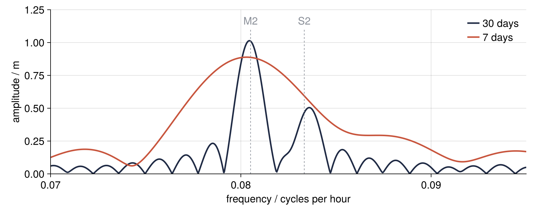
With seven days the two semidiurnal tides fuse into one broad hump, and no amount of cleverness with the spectrum splits it. A least-squares fit told in advance that there are two sinusoids does split it, even from one week, but then the two came from you and not from the data.

The highest frequency you can see. Sampled at the rate \(f_s = 1/\Delta t\), a rhythm at \(f\) and one at \(f_s - f\) take identical values at every sample time, so nothing above \(f_s/2 = 1/(2\Delta t)\), the Nyquist frequency, can be told from its partner below. Hourly readings reach 0.5 cycles per hour, periods of 2 h, far shorter than any tide. The same identity is why the entries \(X_k\) above \(k = N/2\) count as negative frequencies, \((k - N)/T\). A rhythm faster than \(f_s/2\) shows up at its distance from the nearest multiple of \(f_s\): sampled at 1 Hz, a 2.7 Hz vibration reads as 0.3 Hz, not 0.7 Hz.

See it in code

The sweep evaluates the sum once per probe frequency. The fast Fourier transform gets all \(X_k\) in about \(N \log N\) operations, and Julia takes it from FFTW.jl. rfft is the version for real signals: it keeps \(k = 0\) to \(N/2\), 361 entries here, and drops the negative frequencies, which for a real signal are complex conjugates of these. The cell then keeps every local maximum above 0.1 m:

Show code

using FFTW

X = rfft(h)
freq = rfftfreq(length(t), 1.0)            # 1.0 = sample rate, readings per hour
amplitude = 2 .* abs.(X) ./ length(t)      # abs. with the dot: every entry

peaks = [k for k in 2:length(amplitude)-1
         if amplitude[k] > max(amplitude[k-1], amplitude[k+1]) && amplitude[k] > 0.1]
for k in peaks
    @printf("entry %2d   f = %.5f /h   period = %6.2f h   amplitude = %.2f m\n",
            k, freq[k], 1 / freq[k], amplitude[k])
end
@printf("largest entry outside the peaks: %.3f m\n",
        maximum(amplitude[setdiff(2:length(amplitude), peaks)]))

entry 29   f = 0.03889 /h   period =  25.71 h   amplitude = 0.20 m
entry 31   f = 0.04167 /h   period =  24.00 h   amplitude = 0.31 m
entry 59   f = 0.08056 /h   period =  12.41 h   amplitude = 1.00 m
entry 61   f = 0.08333 /h   period =  12.00 h   amplitude = 0.47 m
largest entry outside the peaks: 0.044 m

The truth was 25.82, 23.93, 12.42 and 12.00 h. Only S2 is exact, since 1/12 cycles per hour is a multiple of 1/720; M2 reads 12.41 h and the daily ones 25.71 and 24.00 h, the nearest multiples. A longer record or a fit to the peak shape does better.

Three rules carry over to your own record. The second argument of rfftfreq is the sample rate, not the spacing: a 1 kHz accelerometer needs rfftfreq(n, 1000.0), and 0.001 gives frequencies a million times too small. The Formalization counts from \(k = 0\) and Julia from 1, so every peak sits one entry after its \(k\); take its frequency from the frequency vector, never from the index. The 0.1 m cutoff was set by looking at the amplitudes. The 0.15 m noise per reading averages down to about 0.01 m per frequency, the flank of M2 adds more, and nothing outside the four peaks exceeds 0.044 m. Plot your amplitudes first and set the cutoff well above that floor.

Where it shows up

Tides are one example. Whenever a quantity oscillates and you record it over time or along a distance, asking for its frequencies is asking for its physics.

Engineering and geophysics. To find the resonances of a bridge deck or a turbine blade, an engineer fixes an accelerometer to it, strikes it with an impact hammer, and reads the natural frequencies off the spectrum of the ringing. Seismologists treat ground motion the same way and get from its spectrum both the size of an earthquake and the layering of the crust the waves crossed.
Spectroscopy. An FTIR spectrometer records an interferogram, detector intensity against the position of a moving mirror, and its software turns that into the spectrum by a Fourier transform. In NMR the nuclei ring after the pulse in a decaying free induction decay whose transform is the spectrum, and the resolution rule is why a longer acquisition gives narrower lines.
Crystallography. To a good approximation, the diffraction pattern of a crystal is the squared modulus of the Fourier transform of its electron density, so the phases are gone, as they were for the cosine probe. Getting them back is the phase problem, and methods for solving it earned the 1985 Nobel Prize in Chemistry.
Quantum mechanics. The wavefunction in momentum space is the Fourier transform of the one in position space. The uncertainty principle is the resolution rule with position in place of time: squeeze a wave packet into a length \(L\) and its wavenumbers must range over roughly \(1/L\) or more.
Signal and image processing. A filter against 50 Hz mains hum suppresses the spectrum around 50 Hz and transforms back. JPEG cuts an image into 8 × 8 blocks, transforms each with the discrete cosine transform, a close relative of the Fourier transform, and discards most of the high frequencies.
Biology. Measure the activity of a clock gene every few hours for some days, and the circadian rhythm stands out in the spectrum as a peak at a period of 24 h. EEG bands such as alpha, 8 to 12 Hz, are ranges in the spectrum of the voltage measured on the scalp.

What carries over to every item is the pair of facts this page is built on: the amplitude spectrum says which rhythms are present, and the length of the record limits how close two of them may lie.