Eigenvalues with LinearAlgebra: normal modes of coupled oscillators

The problem: the normal modes of three coupled gliders

Put three gliders of 200 g on an air track, 0.5 m apart, and connect them to each other and to a post at either end with four springs of 10 N/m. Pull the first glider aside with 1 N, wait, and release it: the motion never repeats. Buried in it are three special motions in which all gliders share one frequency, the normal modes. They are the eigenvectors of a matrix, and Julia's standard library LinearAlgebra finds them, with their eigenvalues, in one call.

Newton's law for the displacements of all three gliders reads

\[m\,\ddot{\mathbf x} = -K\,\mathbf x ,\]

with \(m\) the glider mass and \(K\) a symmetric 3 × 3 matrix made of the spring constants. For the gliders the modes are 0.86 Hz, 1.59 Hz, and 2.08 Hz.

Take away the posts and let atoms stand in for the gliders, and the matrix describes CO₂ vibrating along its axis. Fitted to one infrared band of ordinary CO₂, the model puts that band of carbon-13 dioxide at 2282.2 cm⁻¹ (spectroscopists count in wavenumbers, \(\tilde\nu = f/c\)), where 2283.5 cm⁻¹ is measured. The floors of a three-story building follow the same equation.

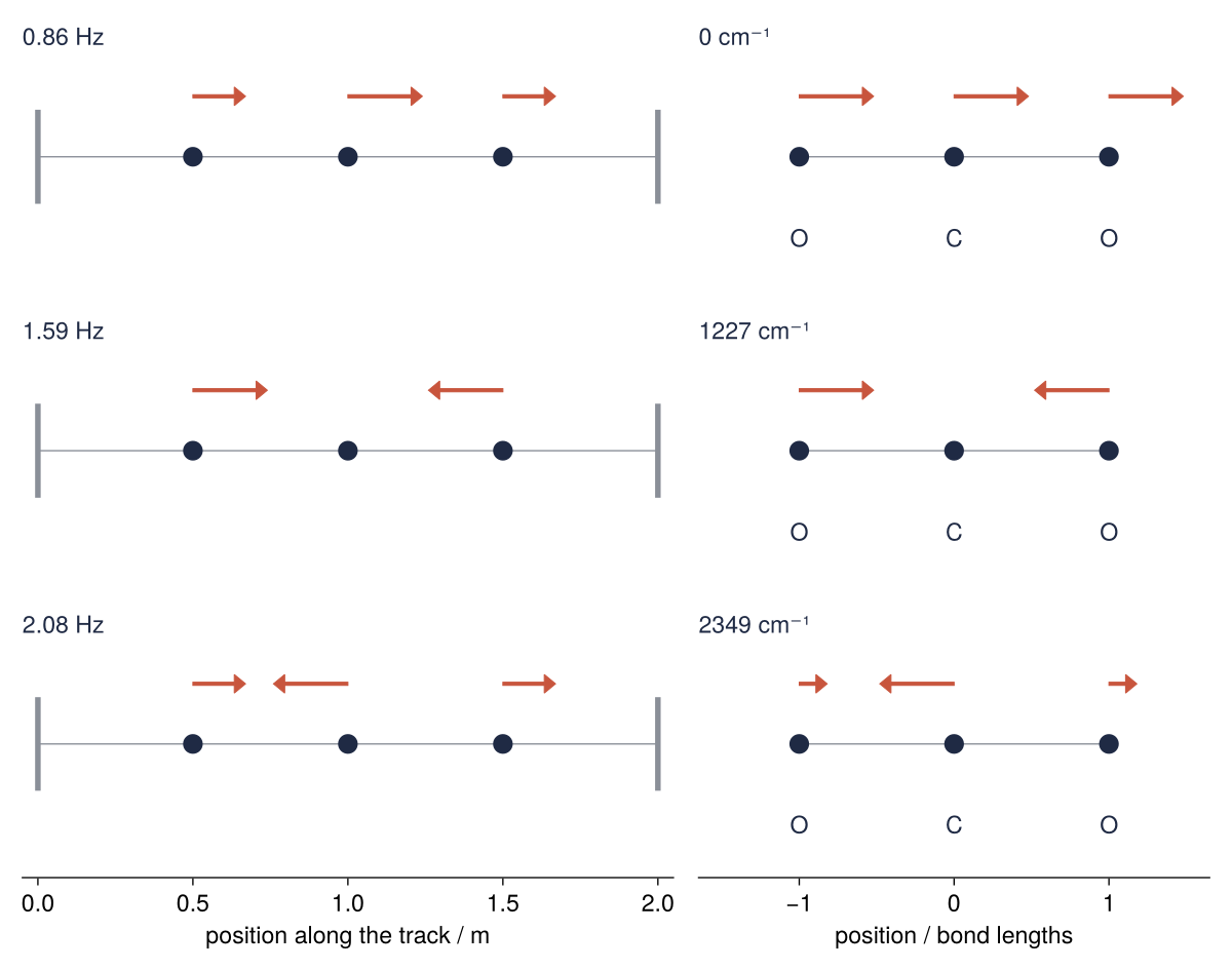
Normal modes of three gliders between two posts (left) and of a CO₂ molecule (right), slowest at the top. Arrows: how far each mass moves in that mode. Frequencies printed in each panel: 0.86, 1.59, 2.08 Hz and 0, 1227, 2349 cm⁻¹.

Each row holds one mode of each system, with arrows for how far every mass travels and the frequency in the corner. All of it is output of eigen, assembled below in six steps from the springs up.

Setup

LinearAlgebra and Printf come with Julia, so CairoMakie is the only package to install. As a yardstick, the cell prints the angular frequency of a single glider on a single spring, 7.071 rad/s.

using LinearAlgebra, Printf, CairoMakie

m = 0.200   # kg, one glider
k = 10.0    # N/m, one spring

const INK, ACCENT, SECOND, MUTED = "#1f2a44", "#c8553d", "#2a7f9e", "#8a8f98"
set_theme!(Theme(                          # the look of every figure below
    size = (770, 396), fontsize = 17,
    palette = (color = [INK, ACCENT, SECOND, MUTED],),
    Axis = (topspinevisible = false, rightspinevisible = false, xgridvisible = true, ygridvisible = true),
    Lines = (linewidth = 2.5,),
))

@printf("one glider on one spring: sqrt(k/m) = %.3f rad/s\n", sqrt(k / m))

one glider on one spring: sqrt(k/m) = 7.071 rad/s

Step 1: Write Newton's equations as one matrix equation

Glider 1 is pulled back by the left spring \(k_1\), stretched by \(x_1\), and forward by the spring \(k_2\) to its neighbor, stretched by \(x_2 - x_1\):

\[m\,\ddot x_1 = -k_1 x_1 + k_2\,(x_2 - x_1) = -(k_1 + k_2)\,x_1 + k_2\,x_2 .\]

Stack one row per glider and you have \(m\ddot{\mathbf x} = -K\mathbf x\). stiffness takes the springs from the left post rightward, 0 marking a free end, and diagm puts the vector of each offset => vector pair on that diagonal. Step 5 reuses it.

function stiffness(springs)
    s = float.(springs)                    # a list of integers still gives a Float64 matrix
    return diagm(0 => s[1:end-1] .+ s[2:end], 1 => -s[2:end-1], -1 => -s[2:end-1])
end

K = stiffness([k, k, k, k])                # N/m; post, glider 1, glider 2, glider 3, post

3×3 Matrix{Float64}:
  20.0  -10.0    0.0
 -10.0   20.0  -10.0
   0.0  -10.0   20.0

Each glider's diagonal entry sums the springs touching it, 20 N/m, and the entries beside it are minus the coupling spring, −10 N/m. That rule builds \(K\) for any spring network, not only chains. \(K\) is symmetric because a spring pulls on both bodies it connects with equal force.

Step 2: Find the starting position with backslash

Held with 1 N, the gliders settle where the springs balance the pull, \(K\mathbf x_0 = \mathbf F\), a linear system for the backslash operator. The check uses ≈, which is isapprox (type \approx, then Tab) and allows for rounding:

F = [1.0, 0.0, 0.0]                        # N, the pull on glider 1
x0 = K \ F                                 # m

@printf("x0 = %.2f, %.2f, %.2f cm\n", (100 .* x0)...)
println("K * x0 ≈ F: ", K * x0 ≈ F)
@printf("left spring %.2f N, right spring %.2f N\n", k * x0[1], k * x0[3])

x0 = 7.50, 5.00, 2.50 cm
K * x0 ≈ F: true
left spring 0.75 N, right spring 0.25 N

Glider 1 ends up 7.5 cm from rest, the others at 5.0 cm and 2.5 cm, and the end springs carry 0.75 N and 0.25 N. Write K \ F, never inv(K) * F. For a dense square matrix like K, backslash uses a triangular factorization called LU and solves with it once. inv starts from the same factorization, then builds the whole inverse matrix and multiplies, all for one right-hand side.

Step 3: Ask eigen for the normal modes

Suppose every glider oscillates at one common frequency with an amplitude of its own, \(\mathbf x(t) = \mathbf a\cos\omega t\). Differentiating twice multiplies by \(-\omega^2\), so Newton's law becomes

\[\frac{K}{m}\,\mathbf a = \omega^2\,\mathbf a .\]

\(K/m\) does not rotate \(\mathbf a\) but only rescales it. Such a vector is an eigenvector of the matrix, and the scale factor, here the squared angular frequency of the mode, is its eigenvalue.

Symmetric declares the matrix symmetric, so eigen uses the symmetric algorithm: real eigenvalues, ascending, and orthonormal eigenvectors (perpendicular, length 1) as columns. The wrapper checks nothing: it reads the upper triangle and takes the lower one as its mirror image. On the bare matrix eigen would test issymmetric itself and choose the same algorithm. eigen returns one object with the fields .values and .vectors, and assigning it to two names unpacks them:

println("issymmetric(K): ", issymmetric(K))
w2, V = eigen(Symmetric(K ./ m))           # eigenvalues are ω², in 1/s^2
ω = sqrt.(w2)                              # rad/s
f = ω ./ 2π                                # Hz
f_exact = sqrt.(k / m .* [2 - sqrt(2), 2, 2 + sqrt(2)]) ./ 2π

@printf("w2    : %7.2f %7.2f %7.2f 1/s^2\n", w2...)
@printf("eigen : %7.3f %7.3f %7.3f Hz\n", f...)
@printf("exact : %7.3f %7.3f %7.3f Hz\n", f_exact...)
round.(V, digits = 3) .+ 0.0               # + 0.0 turns -0.0 into 0.0

issymmetric(K): true
w2    :   29.29  100.00  170.71 1/s^2
eigen :   0.861   1.592   2.079 Hz
exact :   0.861   1.592   2.079 Hz

3×3 Matrix{Float64}:
 0.5     0.707  -0.5
 0.707   0.0     0.707
 0.5    -0.707  -0.5

eigen and the closed form \(\omega^2 = (k/m)\,(2 - \sqrt2,\ 2,\ 2 + \sqrt2)\), a case of the long-chain formula under Variations, agree on every printed digit: 0.861 Hz, 1.592 Hz, 2.079 Hz. The columns of V are the modes. In the slowest all three swing the same way, the middle one with √2 times the amplitude. In the next, glider 2 rests and its neighbors move in opposition. In the fastest, glider 2 swings against both, and in this run its column came out as (−0.5, 0.707, −0.5), which the first pitfall takes up.

Step 4: Check the eigenvectors and rebuild the motion

Column by column \((K/m)\,\mathbf v = \omega^2\mathbf v\), so \((K/m)\,V = V\,\mathrm{Diagonal}(\omega^2)\), and orthonormality is \(V^\mathsf{T}V = I\). V' transposes a real matrix, and I is an identity of any size:

residual = maximum(abs.(K ./ m * V - V * Diagonal(w2)))
@printf("largest entry of (K/m) V - V Diagonal(w2): %.0e 1/s^2\n", residual)
@printf("largest entry of V' V - I:                 %.0e\n", maximum(abs.(V' * V - I)))

largest entry of (K/m) V - V Diagonal(w2): 1e-13 1/s^2
largest entry of V' V - I:                 3e-16

The residual, 10⁻¹³ s⁻², is tiny next to eigenvalues up to 171 s⁻², and orthonormality holds to 3 × 10⁻¹⁶: rounding. Together the checks say \(K/m = V\,\mathrm{Diagonal}(\omega^2)\,V^\mathsf{T}\), so rebuild it:

S = V * Diagonal(w2) * V'                  # K/m put back together from its modes
println("S ≈ K ./ m: ", S ≈ K ./ m, ",  issymmetric(S): ", issymmetric(S))
@printf("largest entry of S - S': %.0e 1/s^2\n", maximum(abs.(S - S')))

S ≈ K ./ m: true,  issymmetric(S): false
largest entry of S - S': 7e-15 1/s^2

S is K ./ m to rounding, yet issymmetric(S) is false in this run: it demands exact equality, and the triangles differ by 7 × 10⁻¹⁵ s⁻². Plain eigen would then take the general path and lose the symmetric guarantees. Wrap whenever the physics says symmetric, as for spring networks and inertia tensors. There the promise is true.

The equation is linear, so after a release from rest the motion is a sum of mode cosines with amplitudes \(c_n\):

\[\mathbf x(t) = \sum_n c_n\,\mathbf v_n \cos\omega_n t .\]

Orthonormal \(\mathbf v_n\) make \(c_n = \mathbf v_n\cdot\mathbf x_0\), all three in V' * x0. cos.(ω .* t') broadcasts three frequencies (a column) against 1001 times (a row) into a 3 × 1001 array, which V * turns into positions. A second release starts at (5, 0, −5) cm, the middle mode alone. The plot follows the CairoMakie pattern: a Figure holds Axis objects placed in its grid as fig[i, 1], and functions ending in ! draw into an existing axis.

c = V' * x0                                # m, amplitude of each mode in the start
@printf("c = %.2f, %.2f, %.2f cm\n", (100 .* c)...)
@printf("frequency ratios: %.3f and %.3f\n", f[2] / f[1], f[3] / f[1])

t = range(0, 10, length = 1001)            # s
x = V * (c .* cos.(ω .* t'))               # m, 3 × 1001
x0_pure = [0.05, 0.0, -0.05]               # m
x_pure = V * ((V' * x0_pure) .* cos.(ω .* t'))

fig = Figure(size = (770, 484))
axes = [Axis(fig[i, 1], ylabel = "displacement / cm", yticks = [-20, 0, 20],
             xticks = 0:2:10, limits = (0, 11.5, -30, 35)) for i in 1:2]
for (ax, xs, color) in [(axes[1], x, INK), (axes[2], x_pure, ACCENT)]
    for (n, offset) in enumerate([20, 0, -20])
        lines!(ax, [0, 10], [offset, offset], color = MUTED, linewidth = 1)   # rest position
        lines!(ax, t, 100 .* xs[n, :] .+ offset, color = color)
        text!(ax, 10.3, offset, text = "glider $n", align = (:left, :center), color = color)
    end
end
text!(axes[2], 0.15, 28, text = @sprintf("%.2f Hz", f[2]), align = (:left, :bottom), color = ACCENT)
linkxaxes!(axes...)
hidexdecorations!(axes[1], grid = false)
axes[2].xlabel = "t / s"
fig

c = 8.54, 3.54, -1.46 cm
frequency ratios: 1.848 and 2.414

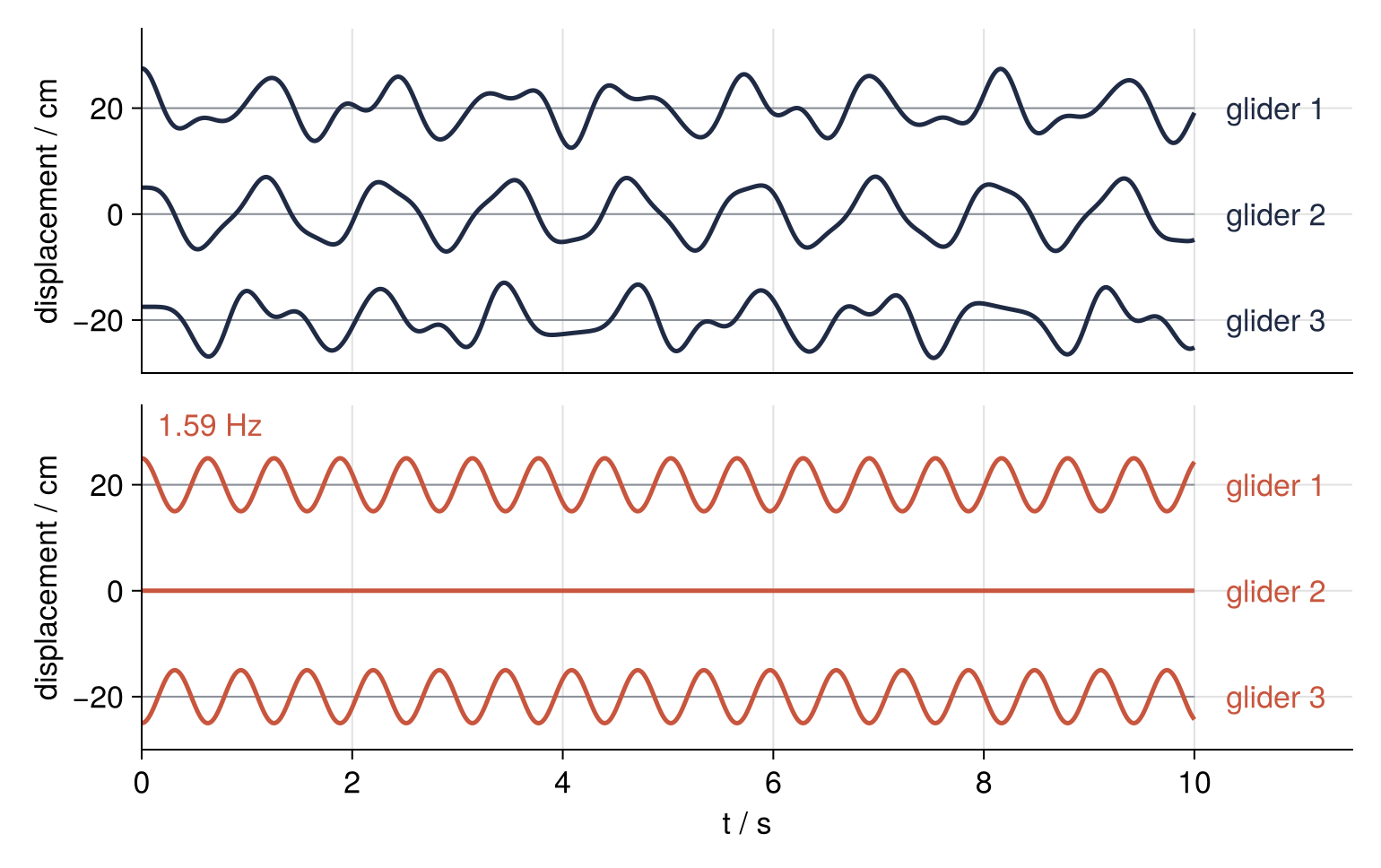
The slowest mode carries 8.54 cm of the start, the others 3.54 cm and −1.46 cm. Curves are offset by 20 cm, gray lines at rest. The frequency ratios, 1.848 and 2.414 (which is 1 + √2), are irrational, so the top panel never repeats. Below, glider 2 sits still while the outer two trace one cosine each at 1.59 Hz. A normal mode looks exactly like that.

Step 5: Solve the generalized eigenproblem when the masses differ

Remove the posts and stiffness builds O=C=O, with bonds as springs of strength 1 and masses in atomic mass units u, so the eigenvalues are plain numbers. Unequal masses make Newton's law \(M\ddot{\mathbf x} = -K\mathbf x\) with \(M\) diagonal. Dividing row \(i\) by \(m_i\) gives \(A = M^{-1}K\), written K1 ./ m_co2 because the column of masses broadcasts along the rows. \(A\) is not symmetric, and the general eigen and the wrapped one no longer agree:

m_co2 = [15.994915, 12.0, 15.994915]       # u: 16O, 12C, 16O (NIST atomic masses)
K1 = stiffness([0, 1, 1, 0])               # no posts, springs of 1
A = K1 ./ m_co2                            # row i divided by m_i

λ, W = eigen(A)
@printf("eigen(A)           : %7.4f %7.4f %7.4f, element type %s\n", λ..., eltype(λ))
@printf("eigen(Symmetric(A)): %7.4f %7.4f %7.4f\n", eigvals(Symmetric(A))...)
@printf("dot product of the first and last vector of eigen(A): %.3f\n", dot(W[:, 1], W[:, 3]))

eigen(A)           : -0.0000  0.0625  0.2292, element type Float64
eigen(Symmetric(A)): -0.0019  0.0625  0.2311
dot product of the first and last vector of eigen(A): -0.127

The general call gets the values right, 0, 0.0625, and 0.2292, sorted by real part as eigen does by default. A matrix that is not symmetric can have complex eigenvalues, but \(M^{-1}K\) shares those of the symmetric \(M^{-1/2}KM^{-1/2}\), and every imaginary part came out exactly zero. The vectors of eigen(A) are not orthogonal (dot product −0.127), so V' * x0 would misassign the amplitudes. The symmetric call, here as eigvals(Symmetric(A)), returns −0.0019 and 0.2311 at the ends without complaint: it mirrored the upper triangle. Julia trusted a false promise.

The cure keeps \(K\) symmetric and passes the masses separately. Step 3's trial cosine turns \(M\ddot{\mathbf x} = -K\mathbf x\) into the generalized eigenproblem

\[K\,\mathbf a = \omega^2 M\,\mathbf a ,\]

which eigen solves with \(M\) as a second argument:

M = Diagonal(m_co2)                        # u
w2_co2, X = eigen(Symmetric(K1), M)        # K a = ω² M a, ascending
@printf("eigen(Symmetric(K1), M): %.4f %.4f %.4f\n", w2_co2...)
@printf("1/m_O = %.4f,  1/m_O + 2/m_C = %.4f\n", 1 / m_co2[1], 1 / m_co2[1] + 2 / m_co2[2])
round.(X, digits = 3) .+ 0.0

eigen(Symmetric(K1), M): 0.0000 0.0625 0.2292
1/m_O = 0.0625,  1/m_O + 2/m_C = 0.2292

3×3 Matrix{Float64}:
 0.151   0.177  -0.092
 0.151   0.0     0.246
 0.151  -0.177  -0.092

The values ascend: 0, then \(1/m_\mathrm{O}\) = 0.0625, the oxygens bouncing on a resting carbon, then \(1/m_\mathrm{O} + 2/m_\mathrm{C}\) = 0.2292. The columns of X are the patterns, normalized so that \(X^\mathsf{T}MX = I\), which makes them orthogonal only with the masses as weights. The amplitudes of a start are therefore X' * M * x0. Displace the first oxygen by 1 and rebuild it both ways:

x0_co2 = [1.0, 0.0, 0.0]
c_co2 = X' * M * x0_co2                    # amplitudes, with the masses as weights
println("X * c_co2 ≈ x0_co2:         ", X * c_co2 ≈ x0_co2)
println("X * (X' * x0_co2) ≈ x0_co2: ", X * (X' * x0_co2) ≈ x0_co2)

X * c_co2 ≈ x0_co2:         true
X * (X' * x0_co2) ≈ x0_co2: false

Only the weighted projection gives the start back. Keep the matrix symmetric, pass the masses, and leave the general call to matrices that cannot be made symmetric, as in damped systems.

Step 6: Read the eigenvalues as a CO₂ spectrum

Column three of X, (−0.092, 0.246, −0.092) in this run, moves the carbon against both oxygens. That is the asymmetric stretch, with the largest eigenvalue, w2_co2[3], and a strong infrared band, so the spring is fitted to it. Its band origin, the vibrational frequency at the center of the band between its rotational lines, is \(\tilde\nu_3 = 2349.1\) cm⁻¹ in ¹²C¹⁶O₂, from the HITRAN line database.

In real units \(K\) scales with the spring \(k\) and \(M\) with \(u = 1.66054 \times 10^{-27}\) kg, so an eigenvalue \(\lambda\) becomes \(\omega^2 = \lambda\,k/u\) and \(k = (2\pi c\,\tilde\nu_3)^2\,u/\lambda_3\). Inside wavenumbers the units are kg and N/m, so eigvals returns \(\omega^2\) in s⁻² directly. The clip max.(w2, 0) is needed: the zero mode can land below zero, like Step 5's −0.0000, and sqrt of a negative number throws a DomainError.

u = 1.66054e-27          # kg, atomic mass constant (CODATA)
c_cm = 2.99792458e10     # cm/s, speed of light, exact in SI
nu3_12 = 2349.1          # cm^-1, band origin of the asymmetric stretch of 12C16O2 (HITRAN lines)
k_bond = (2π * c_cm * nu3_12)^2 * u / w2_co2[3]
@printf("k = %.0f N/m\n", k_bond)

function wavenumbers(masses_u, k_bond)
    w2 = eigvals(Symmetric(stiffness([0, k_bond, k_bond, 0])), Diagonal(masses_u .* u))
    return sqrt.(max.(w2, 0)) ./ (2π * c_cm)
end

m_13 = [15.994915, 13.003355, 15.994915]   # u: 16O, 13C, 16O (NIST atomic masses)
nu3_13_measured = 2283.5                   # cm^-1, band origin of the same band in 13C16O2 (HITRAN lines)
@printf("12C16O2: %.1f, %.1f, %.1f cm^-1\n", wavenumbers(m_co2, k_bond)...)
@printf("13C16O2: model %.1f cm^-1, measured %.1f cm^-1\n", wavenumbers(m_13, k_bond)[3], nu3_13_measured)

k = 1419 N/m
12C16O2: 0.0, 1226.9, 2349.1 cm^-1
13C16O2: model 2282.2 cm^-1, measured 2283.5 cm^-1

The spring is 1419 N/m. The 0 is the molecule translating as a whole. At 1226.9 cm⁻¹ the oxygens move against each other around a still carbon, a symmetric stretch that leaves the dipole moment unchanged and has no infrared line to compare with. The 2349.1 cm⁻¹ went in through the spring and proves nothing.

Carbon-13 is the test: its bonds and spring are unchanged, and the model predicts 2282.2 cm⁻¹ where 2283.5 cm⁻¹ is measured. The spring drops out of that comparison, so the agreement tests the mass weighting, not the fit. The leftover 1.3 cm⁻¹ is anharmonicity: a bond is a spring only approximately.

For the drawing, sign_fixed picks one version of each eigenvector, defined only up to a factor: largest entry 1, first entry positive. draw_mode! draws one panel, the masses at rest with an arrow for each one that moves.

function sign_fixed(v)
    v = v ./ maximum(abs, v)
    return v[1] > 0 ? v : -v
end

function draw_mode!(ax, rest, mode, scale, label; names = (), posts = ())
    ends = isempty(posts) ? (rest[1], rest[end]) : posts
    lines!(ax, collect(ends), [0.0, 0.0], color = MUTED, linewidth = 1)    # the springs
    for p in posts
        lines!(ax, [p, p], [-0.35, 0.35], color = MUTED, linewidth = 4)
    end
    scatter!(ax, rest, zeros(3), color = INK, markersize = 20)
    for (r, d) in zip(rest, sign_fixed(mode))
        abs(d) > 1e-6 || continue                                         # a mass at rest gets no arrow
        arrows2d!(ax, [Point2f(r, 0.45)], [Vec2f(scale * d, 0)], color = ACCENT)
    end
    for (r, name) in zip(rest, names)
        text!(ax, r, -0.5, text = name, align = (:center, :top), color = INK)
    end
    text!(ax, 0, 1, text = label, space = :relative, align = (:left, :top), color = INK)  # axis fractions
    ylims!(ax, -1, 1)
    hideydecorations!(ax)
    ax.leftspinevisible = false
    ax.xgridvisible = false                                               # grid lines would cross the labels
end

nu = wavenumbers(m_co2, k_bond)
fig = Figure(size = (880, 693))
axes = [Axis(fig[n, j]) for n in 1:3, j in 1:2]
for n in 1:3
    draw_mode!(axes[n, 1], [0.5, 1.0, 1.5], V[:, n], 0.24, @sprintf("%.2f Hz", f[n]), posts = (0.0, 2.0))
    draw_mode!(axes[n, 2], [-1.0, 0.0, 1.0], X[:, n], 0.48, @sprintf("%.0f cm⁻¹", nu[n]), names = ("O", "C", "O"))
end
for j in 1:2                                                              # one x axis per column
    linkxaxes!(axes[:, j]...)
    for n in 1:2
        hidexdecorations!(axes[n, j], grid = false)
        axes[n, j].bottomspinevisible = false
    end
end
axes[3, 1].xlabel = "position along the track / m"
axes[3, 2].xlabel = "position / bond lengths"
xlims!(axes[3, 1], -0.05, 2.05)
xlims!(axes[3, 2], -1.65, 1.65)
colsize!(fig.layout, 1, Auto(4.2))                                        # widths follow the x ranges
colsize!(fig.layout, 2, Auto(3.3))
fig

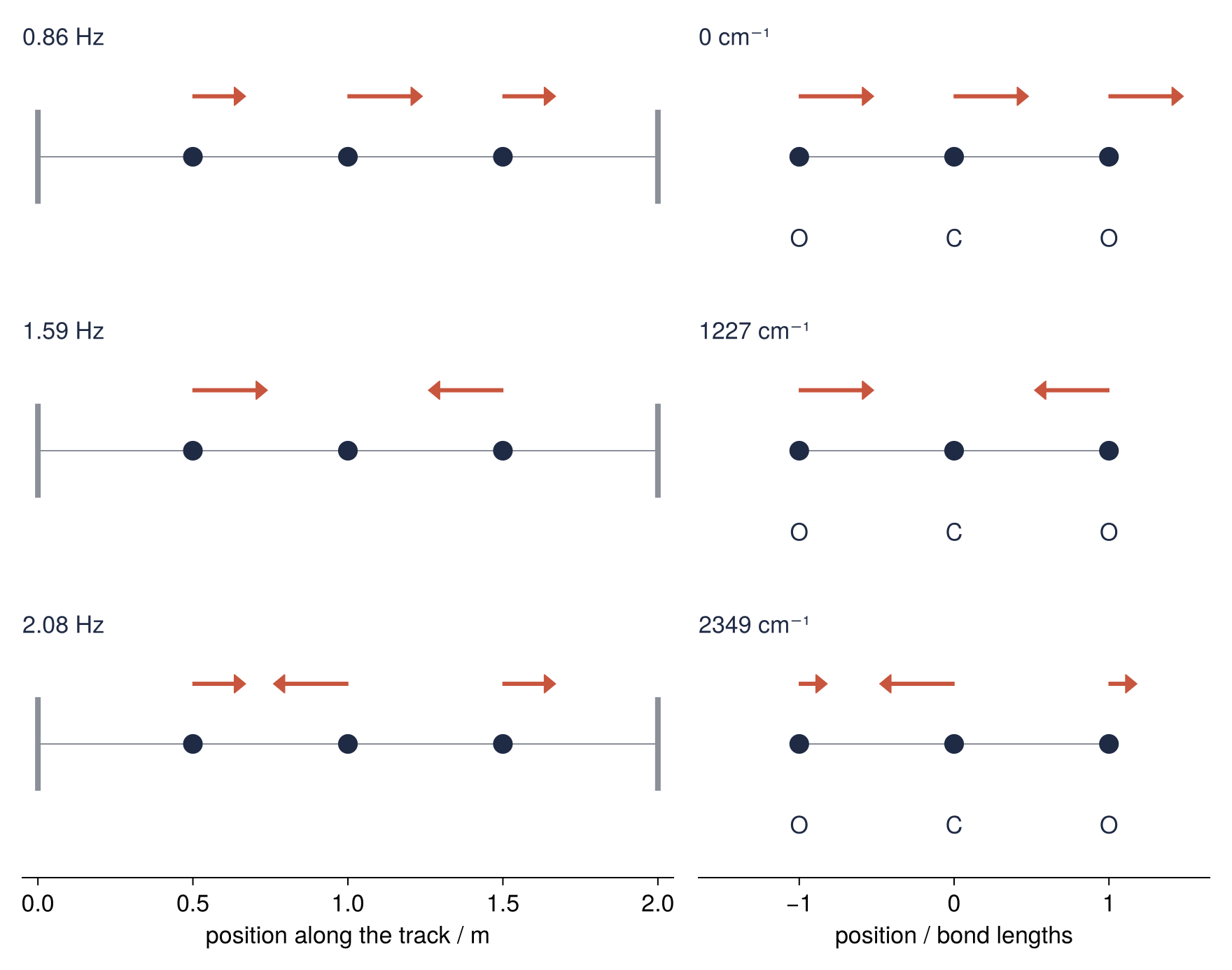
Row for row, the arrows of both systems point alike. In the fastest mode the carbon moves 0.246 against 0.092 for each oxygen, 2.67 times as far, which keeps the center of mass in place.

Pitfalls

Comparing eigenvectors by sign or length. Step 3 returned the fastest mode as (−0.5, 0.707, −0.5), and checking it against the textbook vector \((1, -\sqrt2, 1)/2\) fails. Any multiple of an eigenvector, \(-\mathbf v\) included, is an eigenvector too. eigen normalizes to length 1 and keeps whatever sign the algorithm arrived at, which can change with a library update and flip your plot. The generalized call normalizes differently, to \(X^\mathsf{T}MX = I\), so its columns are not of length 1. Check the defining properties instead:

textbook = [1, -sqrt(2), 1] / 2            # the fastest glider mode at length 1
println("V[:, 3] ≈ textbook:                ", V[:, 3] ≈ textbook)
println("equal up to sign:                  ", abs(dot(V[:, 3], textbook)) ≈ 1)
println("K1 * X ≈ M * X * Diagonal(w2_co2): ", K1 * X ≈ M * X * Diagonal(w2_co2))
println("X' * M * X ≈ I:                    ", X' * M * X ≈ I)

V[:, 3] ≈ textbook:                false
equal up to sign:                  true
K1 * X ≈ M * X * Diagonal(w2_co2): true
X' * M * X ≈ I:                    true

Compare up to sign, as in the second check, and choose a sign before plotting, which is what sign_fixed does.

Taking rows for modes. You notice it when a supposed mode fails its own eigenvalue check. eigen stores the vectors as the columns of its field .vectors, unpacked here into V, and V[1, :] is a row. With the gliders this goes unnoticed for a while, since the first row of V, (0.5, 0.707, −0.5), looks like the slowest mode with one sign flipped. With the molecule a row of X is no mode of anything. Index columns, V[:, n], or loop over zip(w2, eachcol(V)) to get each value with its vector.

A free molecule has no static answer. Ask backslash where the molecule settles under a pull on one oxygen, as Step 2 did for the gliders:

try
    K1 \ [1.0, 0.0, 0.0]
catch err
    println(err)
end

SingularException(3)

Without posts, moving the whole molecule stretches no spring. K1 therefore has a zero eigenvalue and cannot be inverted, and under a constant force there is no equilibrium. Anchor the system first, with a spring to a wall or by holding one atom fixed and deleting its row and column.

Variations

A three-story building. stiffness([k1, k2, k3, 0]), with the ground as the left post and nothing above the roof. The floor masses go into Step 5's call as Diagonal(m_floors), and the amplitudes of an initial sway are X' * M * x0.
Driven at one frequency. A drive \(F\cos\Omega t\) on glider 1 and a steady state \(\mathbf x\cos\Omega t\) give \((K - \Omega^2 M)\,\mathbf x = \mathbf F\), one backslash per \(\Omega\). The amplitude diverges as \(\Omega/2\pi\) hits 0.86 Hz, 1.59 Hz, or 2.08 Hz.
A long chain. With stiffness(fill(k, N + 1)) and \(N\) gliders the angular frequencies are \(\omega_n = 2\sqrt{k/m}\,\sin\big(n\pi/(2N + 2)\big)\), 5.41 rad/s or 0.861 Hz for \(N = 3\), \(n = 1\), and each mode is a sine sampled at the gliders: a discrete string, and the idea behind finite differences for PDEs. At large \(N\), SymTridiagonal(K) keeps just the three nonzero diagonals, and eigen accepts that type.
Principal axes. Inertia tensors and covariance matrices are symmetric too, and eigen(Symmetric(...)) hands back their principal axes as columns and the principal moments or variances as values. A planned Concept tutorial on eigenvalues explains why one call fits all of these.

Cheat sheet

x = K \ F                                    # K x = F; not inv(K) * F
w2, V = eigen(Symmetric(S))                  # promise: S symmetric; ascending, real, orthonormal
v = V[:, n]                                  # the n-th eigenvector is a column
S * V ≈ V * Diagonal(w2)                     # check S v = λ v, all columns at once
V' * V ≈ I                                   # check orthonormality
c = V' * x0                                  # amplitude of each mode in x0
w2, X = eigen(Symmetric(K), M)               # K a = ω² M a, M = Diagonal(m); X' * M * X ≈ I
c = X' * M * x0                              # amplitudes with masses, not X' * x0
ω = sqrt.(max.(w2, 0))                       # eigenvalues are ω²; clip rounding, sqrt(-x) throws
λ, W = eigen(A)                              # general A: sorted by real part, real or complex