HypothesisTests.jl from the ground up: do two samples really differ?

The problem: is a 4.6 % higher yield real?

Twenty-four batches of a preparation are made, half with the standard protocol A and half with a modified protocol B, and every batch is weighed. Protocol B gives 51.60 mg on average, 2.26 mg above A, a gain of 4.6 %. Yet within each protocol the batches scatter around their mean by 2.3 to 2.5 mg, more than the gain. Did the modification help, or did twenty-four noisy numbers open the gap on their own? HypothesisTests.jl, the JuliaStats package for classical tests, answers that, with StatsBase to describe the samples and Distributions for the t distribution underneath. To a chemist the numbers are a synthesis yield, to a biologist protein from a culture; below they are just the yield.

Six steps get you the answer: a description of both samples, an interval for each mean, the test of the difference, its size with an interval, a count of what chance alone produces, and a check of every verdict. That last check is possible because the data are simulated: the true means are set in the setup and stay hidden from every step but the last.

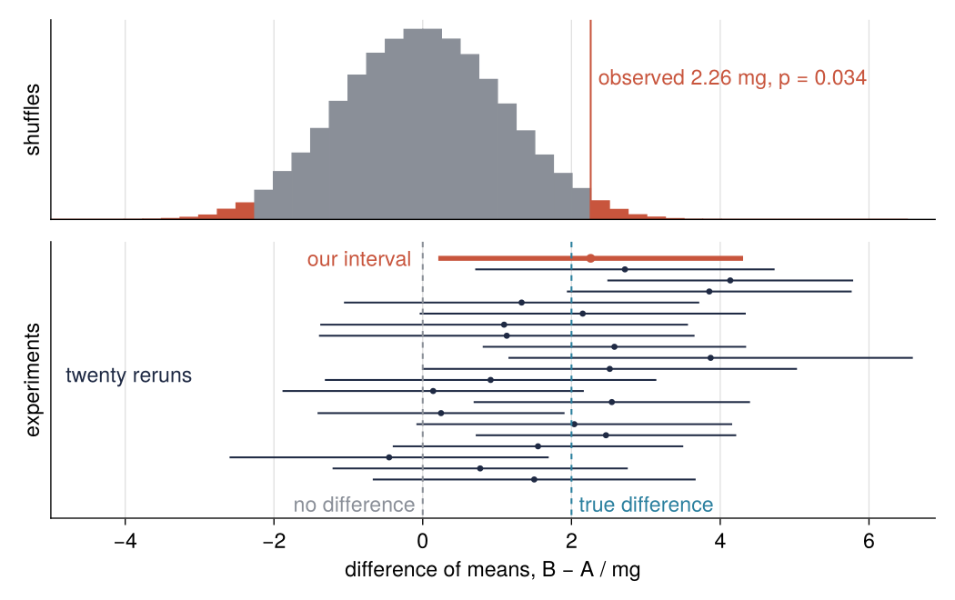
The top panel shuffles the labels A and B and shows the differences that chance produces when the protocol does nothing; the observed 2.26 mg sits out in the tail. The bottom panel shows our interval for B − A together with the intervals of twenty repeats of the experiment under the same truth. The shuffles are Step 5, the reruns Step 6. The verdict in advance: a gain this large rarely arises by chance, and the 95 % interval for the gain runs from 0.4 % to 8.7 %.

Setup

Install the packages once with import Pkg; Pkg.add(["HypothesisTests", "StatsBase", "Distributions", "CairoMakie"]); Statistics, Random, and Printf ship with Julia. Every random number below comes from one Xoshiro generator, Julia's default algorithm, seeded so that each run draws the same yields:

using HypothesisTests, Statistics, StatsBase, Distributions, Random, Printf, CairoMakie

# the truth, which a real experiment never shows you; used again only in Step 6
mu_A, mu_B = 50.0, 52.0     # true mean yields, mg
sigma = 2.5                 # true batch-to-batch scatter, mg
n = 12                      # batches per protocol

rng = Xoshiro(1968)
a = round.(rand(rng, Normal(mu_A, sigma), n), digits = 1)     # the balance reads 0.1 mg
b = round.(rand(rng, Normal(mu_B, sigma), n), digits = 1)

const INK, ACCENT, SECOND, MUTED = "#1f2a44", "#c8553d", "#2a7f9e", "#8a8f98"
set_theme!(Theme(
    size = (770, 396), fontsize = 17,
    palette = (color = [INK, ACCENT, SECOND, MUTED],),
    Axis = (topspinevisible = false, rightspinevisible = false, xgridvisible = true, ygridvisible = true),
    Lines = (linewidth = 2.5,),
))

println("A: ", a)
println("B: ", b)

A: [51.2, 49.0, 48.4, 49.6, 49.9, 50.6, 52.8, 47.1, 44.9, 52.0, 50.1, 46.5]
B: [54.3, 53.7, 49.4, 52.6, 52.6, 51.0, 48.2, 55.7, 53.1, 51.2, 47.4, 50.0]

Step 1: Describe each sample with describe and StatsBase

StatsBase's describe prints what a lab notebook wants about one sample: size, mean, standard deviation, extremes, quartiles, and median.

describe(a)

Summary Stats:
Length:         12
Missing Count:  0
Mean:           49.341667
Std. Deviation: 2.312990
Minimum:        44.900000
1st Quartile:   48.075000
Median:         49.750000
3rd Quartile:   50.750000
Maximum:        52.800000
Type:           Float64

For both samples side by side, take the numbers one function at a time and format them with @printf, the C-style formatted print from Printf:

for (name, x) in [("A", a), ("B", b)]
    @printf("%s: mean %5.2f mg   variance %4.2f mg²   sd %4.2f mg   sem %4.2f mg   skewness %5.2f\n",
            name, mean(x), var(x), std(x), sem(x), skewness(x))
end
@printf("std(a) = %.2f mg   std(a; corrected = false) = %.2f mg\n", std(a), std(a; corrected = false))

A: mean 49.34 mg   variance 5.35 mg²   sd 2.31 mg   sem 0.67 mg   skewness -0.41
B: mean 51.60 mg   variance 6.35 mg²   sd 2.52 mg   sem 0.73 mg   skewness -0.15
std(a) = 2.31 mg   std(a; corrected = false) = 2.21 mg

The variance is the mean squared distance from the mean, divided by n − 1 rather than n; its square root, the standard deviation (sd), is in mg again. Divide the sd by √n and you have the standard error of the mean (sem), 0.67 mg for A, where the sd is 2.31 mg: it is the scatter of the mean of twelve batches, not of one batch. A symmetric sample has zero skewness, so −0.41 and −0.15 mean that neither sample trails off to one side; Pitfall 2 says what counts as large at twelve values.

Julia's std and var divide by n − 1 already. corrected = false divides by n, 2.21 mg here, and is meant for a whole population, never for a sample you measured.

Step 2: Ask the t distribution for a confidence interval

How far from 49.34 mg can the true mean of A lie? For normally scattered batches, the ratio (mean − true mean) / sem, the miss of the sample mean in standard errors, is distributed as Student's t with 11 degrees of freedom, n − 1: the mean uses up one of the twelve values, and eleven remain for the scatter. The 95 % interval is mean ± c × sem, with 2.5 % of the distribution above c and, by symmetry, 2.5 % below −c. So c is the 0.975 quantile.

TDist(11) is that distribution in Distributions.jl. quantile(d, q) is the point with a fraction q of the distribution to its left, cdf(d, x) the fraction left of x, and ccdf(d, x), the complementary cdf, the fraction right of x, the tail area:

t11 = TDist(11)
c = quantile(t11, 0.975)
@printf("quantile(t11, 0.975) = %.3f   cdf(t11, %.3f) = %.3f   ccdf(t11, %.3f) = %.3f\n",
        c, c, cdf(t11, c), c, ccdf(t11, c))
@printf("normal distribution: quantile(Normal(), 0.975) = %.3f\n", quantile(Normal(), 0.975))

quantile(t11, 0.975) = 2.201   cdf(t11, 2.201) = 0.975   ccdf(t11, 2.201) = 0.025
normal distribution: quantile(Normal(), 0.975) = 1.960

One cut c, read as a point, as the area to its left, and as the area to its right. The t value, 2.201, exceeds the normal 1.960 because the sem is computed from the yields themselves and scatters too.

confint applied to HypothesisTests' one-sample t-test object, OneSampleTTest(x), returns the same interval at its default level of 95 %. What the object tests is the subject of Step 3; here only its interval matters:

half_A = c * sem(a)
@printf("A by hand: %.2f ± %.2f = %.2f to %.2f mg\n", mean(a), half_A, mean(a) - half_A, mean(a) + half_A)
for (name, x) in [("A", a), ("B", b)]
    low, high = confint(OneSampleTTest(x))
    @printf("%s confint:  %.2f ± %.2f = %.2f to %.2f mg\n", name, mean(x), (high - low) / 2, low, high)
end

A by hand: 49.34 ± 1.47 = 47.87 to 50.81 mg
A confint:  49.34 ± 1.47 = 47.87 to 50.81 mg
B confint:  51.60 ± 1.60 = 50.00 to 53.20 mg

That is a confidence interval. Its 95 % belongs to the recipe, not to this one interval: of many experiments, each with an interval built this way, 95 % catch the true mean, and this interval either does or does not. Step 6 puts that to the test.

Copy

fig = Figure(size = (550, 396))
ax = Axis(fig[1, 1], ylabel = "yield / mg", xgridvisible = false,
          xticks = ([0, 1], ["standard (A)", "modified (B)"]))
offsets = range(-0.12, 0.12, length = n)          # fixed spread in batch order, so no dot hides another
bounds = [confint(OneSampleTTest(x)) for x in (a, b)]
band!(ax, [0.3, 1.3], fill(bounds[2][1], 2), fill(bounds[1][2], 2), color = (MUTED, 0.3))   # the overlap
for (k, x) in enumerate((a, b))
    scatter!(ax, (k - 1) .+ offsets, x, color = INK, markersize = 7)
    low, high = bounds[k]
    errorbars!(ax, [k - 0.7], [mean(x)], [mean(x) - low], [high - mean(x)], color = ACCENT, whiskerwidth = 8)
    scatter!(ax, [k - 0.7], [mean(x)], color = ACCENT, markersize = 10)
end
xlims!(ax, -0.4, 1.6)
fig

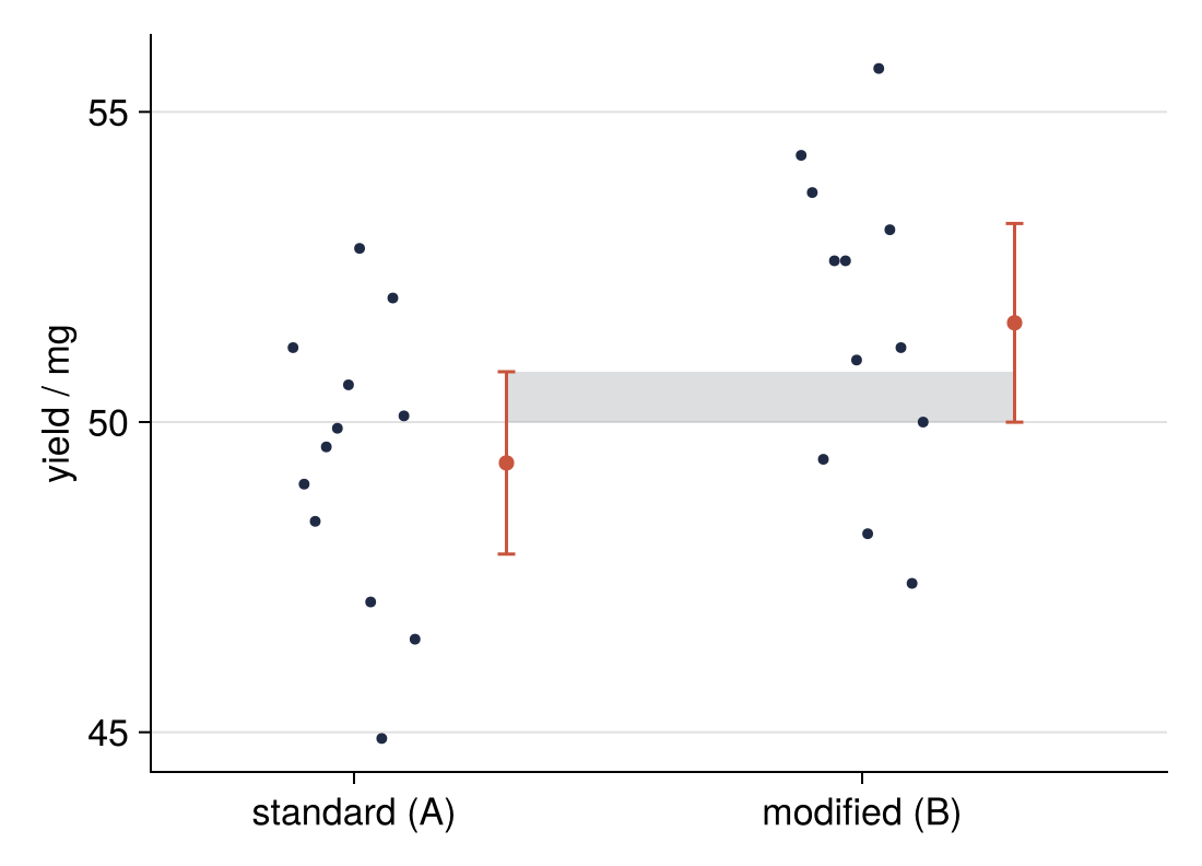
Each dot is a batch, and the red marks are the means with their 95 % intervals. A's and B's batches mostly cover the same range, and the intervals share 50.00 to 50.81 mg. Step 4 settles whether that overlap allows a difference of zero.

Step 3: Test the difference with UnequalVarianceTTest

UnequalVarianceTTest(b, a) compares the means of two independent samples. B goes first because the argument order is the sign: the test works with mean(b) − mean(a). It divides that difference by its standard error,

with sample means \(\bar a, \bar b\), standard deviations \(s_a, s_b\), and batch counts \(n_a, n_b\). Displayed, the test object prints its own report:

res = UnequalVarianceTTest(b, a)

Two sample t-test (unequal variance)
------------------------------------
Population details:
    parameter of interest:   Mean difference
    value under h_0:         0
    point estimate:          2.25833
    95% confidence interval: (0.2094, 4.307)

Test summary:
    outcome with 95% confidence: reject h_0
    two-sided p-value:           0.0323

Details:
    number of observations:   [12,12]
    t-statistic:              2.28684
    degrees of freedom:       21.8396
    empirical standard error: 0.987533

The point estimate is the difference, 2.258 mg, with its 95 % interval, the subject of Step 4. h_0 is the null hypothesis: the protocol has no effect, and the true difference is 0. The p-value, 0.0323, is how often t, the difference in units of its standard error, would reach 2.29 or more in size, of either sign, if h_0 held; it is not the probability that h_0 is true. Below come t, the degrees of freedom, and the standard error. The last line applies a threshold set by convention, the significance level 0.05: "reject h_0" only means p ≤ 0.05, and its "95% confidence" is 1 − 0.05, a property of the recipe as in Step 2, not a 95 % chance that the effect is real.

The fields hold the same numbers, and pvalue computes p from them. The cell checks p with Step 2's ccdf and runs EqualVarianceTTest, Student's older test, for comparison:

@printf("xbar = %.3f mg   stderr = %.3f mg   t = %.2f   df = %.1f   p = %.4f\n",
        res.xbar, res.stderr, res.t, res.df, pvalue(res))
@printf("2 × ccdf(TDist(df), |t|) = %.4f\n", 2 * ccdf(TDist(res.df), abs(res.t)))
student = EqualVarianceTTest(b, a)
@printf("Student's test: t = %.2f   df = %d   p = %.4f\n", student.t, student.df, pvalue(student))

xbar = 2.258 mg   stderr = 0.988 mg   t = 2.29   df = 21.8   p = 0.0323
2 × ccdf(TDist(df), |t|) = 0.0323
Student's test: t = 2.29   df = 22   p = 0.0322

Step 2's ccdf gives p back: the tails beyond ±2.29 hold 3.23 % of the t distribution. A t-test is no more than that, a statistic and its tail area. Welch's test, which UnequalVarianceTTest runs, uses an effective number of degrees of freedom between 11 and 22, here 21.8, from an approximation that fits one t distribution to two unequal scatters. Student's test assumes equal scatters and, for groups of equal size, changes only the degrees of freedom, to 22, and p by 0.0001. Welch's test costs next to nothing when the scatters agree. Make it your default.

Step 2's OneSampleTTest(x) is the same kind of object, testing a true mean of 0 mg. For a yield its p means nothing, but its interval does not depend on h_0.

Step 4: Report the effect size with a confidence interval

The effect size is how large the difference is, in the unit measured: B − A = 2.26 mg, or 4.6 % of A. Cohen's d, in the variations, measures it in units of the scatter instead. confint(res) gives its interval, built like Step 2's: the difference ± c × its standard error, with c now the 0.975 quantile for 21.8 degrees of freedom.

ci = confint(res)
delta = res.xbar
c_diff = quantile(TDist(res.df), 0.975)
half_diff = c_diff * res.stderr
@printf("c = %.3f   by hand: %.2f ± %.2f = %.2f to %.2f mg\n",
        c_diff, delta, half_diff, delta - half_diff, delta + half_diff)
@printf("confint(res):              %.2f to %.2f mg\n", ci[1], ci[2])

c = 2.075   by hand: 2.26 ± 2.05 = 0.21 to 4.31 mg
confint(res):              0.21 to 4.31 mg

Zero lies outside the interval exactly when p < 0.05: both compare |t| = 2.29 with the cut 2.075. That leaves Step 2's overlap. Two intervals overlap when the gap between the means is less than their half-widths added; the difference's interval excludes zero when the gap exceeds its own half-width, 2.05 mg. The cell adds the half-widths, and the standard errors directly and in squares:

half_B = c * sem(b)
@printf("half-widths of A and B added: %.2f + %.2f = %.2f mg\n", half_A, half_B, half_A + half_B)
@printf("standard errors added: %.3f + %.3f = %.3f mg   in squares: √(%.3f² + %.3f²) = %.3f mg\n",
        sem(a), sem(b), sem(a) + sem(b), sem(a), sem(b), sqrt(sem(a)^2 + sem(b)^2))

half-widths of A and B added: 1.47 + 1.60 = 3.07 mg
standard errors added: 0.668 + 0.728 = 1.395 mg   in squares: √(0.668² + 0.728²) = 0.988 mg

The observed 2.26 mg lies between: above 2.05 mg, so zero is excluded, and below 3.07 mg, so A's and B's intervals overlap. Both can hold because standard errors combine in squares, to 0.988 mg, Step 3's res.stderr, not to 1.395 mg. Overlapping intervals never mean "no difference".

The line to report, with percentages relative to A's mean:

pct = 100 / mean(a)
@printf("B − A = %.2f mg (%.1f %% of A), 95 %% CI %.2f to %.2f mg (%.1f %% to %.1f %%), Welch p = %.3f\n",
        delta, delta * pct, ci[1], ci[2], ci[1] * pct, ci[2] * pct, pvalue(res))

B − A = 2.26 mg (4.6 % of A), 95 % CI 0.21 to 4.31 mg (0.4 % to 8.7 %), Welch p = 0.032

A 0.4 % gain would not justify changing a protocol; 8.7 % would. The result is that whole range, and p adds only that it stops short of zero. The same pattern, a value ± a multiple of its standard error, returns for fitted parameters in Fit a curve with error bars and draw a confidence band in Julia, where the uncertainties are known beforehand and the multiple comes from the normal distribution.

Step 5: Simulate the null by shuffling the labels

Shuffling answers the same question without distribution theory. If protocol B changes nothing, the labels are an accident, and every division of the 24 yields into two sets of twelve was as likely as the one in the lab book. There are binomial(24, 12) = 2,704,156 of them. ApproximatePermutationTest draws 100,000 at random instead of all, hence "approximate". Its fourth argument is a per-group statistic: on each shuffle the test takes mean of the first twelve values minus mean of the last twelve.

perm = ApproximatePermutationTest(rng, b, a, mean, 100_000)
null = perm.samples          # the difference of means for every shuffle
@printf("observed %.3f mg   of %d splits   sd of the shuffles %.2f mg\n",
        perm.observation, binomial(24, 12), std(null))
@printf("shuffles with B − A ≥ +%.2f mg: %.2f %%   ≤ −%.2f mg: %.2f %%\n",
        delta, 100 * mean(null .>= delta), delta, 100 * mean(null .<= -delta))
@printf("pvalue(perm) = %.4f\n", pvalue(perm))

observed 2.258 mg   of 2704156 splits   sd of the shuffles 1.08 mg
shuffles with B − A ≥ +2.26 mg: 1.71 %   ≤ −2.26 mg: 1.65 %
pvalue(perm) = 0.0336

perm.samples is the null distribution, the differences chance produces when the protocol does nothing; the opening figure's top panel is its histogram. The cell does not end on perm, whose display reports the point estimate as NaN and shows only the first and last ten shuffles. They scatter by 1.08 mg, 1.71 % reach +2.26 mg and 1.65 % reach −2.26 mg, and pvalue adds the tails to 3.36 %, against the t-test's 3.23 %. A brute-force count agrees with a formula, which is the best reason to trust the formula.

pvalue is the plain share k/N of the N shuffles that are at least as extreme; some texts use (k + 1)/(N + 1) to count the observed split itself. With too few shuffles it returns exactly 0; report p < 1/(number of shuffles) then, never p = 0.

Step 6: Check the verdict against the truth

The setup's constants are allowed back now. B − A is truly 2.0 mg; does Step 4's interval catch it?

true_diff = mu_B - mu_A
println(ci[1] <= true_diff <= ci[2])

true

One experiment proves little about a method, so rerun repeats ours 10,000 times with the same truth. [... for _ in 1:R] is a comprehension, a loop inside brackets that collects its results into a vector. The dot in UnequalVarianceTTest.(B, A) broadcasts as it does for any function of two arguments: it pairs the i-th vector of B with the i-th of A and returns 10,000 tests.

function rerun(n; R = 10_000)
    A = [rand(rng, Normal(mu_A, sigma), n) for _ in 1:R]
    B = [rand(rng, Normal(mu_B, sigma), n) for _ in 1:R]
    return A, B, UnequalVarianceTTest.(B, A)
end

A, B, tests = rerun(n)
ps, cis = pvalue.(tests), confint.(tests)
covers = [low <= true_diff <= high for (low, high) in cis]
@printf("runs with p < 0.05:          %.1f %%\n", 100 * mean(ps .< 0.05))
@printf("intervals containing 2.0 mg: %.1f %%\n", 100 * mean(covers))
@printf("first 20 runs: %d contain 2.0 mg, %d lie entirely above zero\n",
        count(covers[1:20]), count(first.(cis[1:20]) .> 0))

runs with p < 0.05:          46.7 %
intervals containing 2.0 mg: 95.5 %
first 20 runs: 17 contain 2.0 mg, 7 lie entirely above zero

95.5 % of the intervals contain the true difference: Step 2's meaning of 95 %, checked. But p < 0.05 comes out in only 46.7 % of the runs. That share is the power, the chance that twelve batches per protocol notice a gain that truly exists, and at twelve batches it is below even odds. I chose the seed so that our experiment is among the 46.7 %.

Copy

fig = Figure(size = (770, 484))
top = Axis(fig[1, 1], ylabel = "shuffles", yticksvisible = false, yticklabelsvisible = false,
           ygridvisible = false, xticks = -4:2:6)
bottom = Axis(fig[2, 1], xlabel = "difference of means, B − A / mg", ylabel = "experiments",
              yticksvisible = false, yticklabelsvisible = false, ygridvisible = false,
              xticks = -4:2:6)
linkxaxes!(top, bottom)
hidexdecorations!(top, grid = false)

# top: the null distribution, with bin edges on ±2.26 mg so that the tails shade cleanly
w = delta / 9
edges = w .* (-21:26)
counts = fit(Histogram, null, edges).weights
centers = edges[1:end-1] .+ w / 2
shade = [abs(x) > delta ? ACCENT : MUTED for x in centers]
barplot!(top, centers, counts, width = w, gap = 0, color = shade,
         strokewidth = 1, strokecolor = shade)     # stroke in the fill color: no seams between bars
vlines!(top, delta, color = ACCENT, linewidth = 1.5)
text!(top, delta, 0.75 * maximum(counts), text = @sprintf("observed %.2f mg, p = %.3f", delta, pvalue(perm)),
      offset = (6, 0), align = (:left, :center), color = ACCENT)

# bottom: our interval in row 0, then the first twenty reruns
rows = 1:20
lines!(bottom, [ci[1], ci[2]], [0, 0], color = ACCENT, linewidth = 4)
scatter!(bottom, [delta], [0], color = ACCENT, markersize = 10)
rangebars!(bottom, rows, first.(cis[rows]), last.(cis[rows]), direction = :x,
           color = INK, linewidth = 1.5, whiskerwidth = 0)
scatter!(bottom, [tests[k].xbar for k in rows], rows, color = INK, markersize = 7)
vlines!(bottom, true_diff, color = SECOND, linewidth = 1.5, linestyle = :dash)
vlines!(bottom, 0, color = MUTED, linewidth = 1.5, linestyle = :dash)
text!(bottom, true_diff + 0.1, 22.2, text = "true difference", color = SECOND, align = (:left, :center))
text!(bottom, -0.1, 22.2, text = "no difference", color = MUTED, align = (:right, :center))
text!(bottom, -0.15, 0, text = "our interval", color = ACCENT, align = (:right, :center))
text!(bottom, -4.8, 10.5, text = "twenty reruns", color = INK, align = (:left, :center))
xlims!(bottom, -5, max(6.5, maximum(last.(cis[rows])) + 0.3))   # no interval cut off
ylims!(top, 0, nothing)                    # bars stand on the axis
ylims!(bottom, 23.5, -1.5)                 # reversed: our interval on top
rowsize!(fig.layout, 1, Relative(0.42))
fig

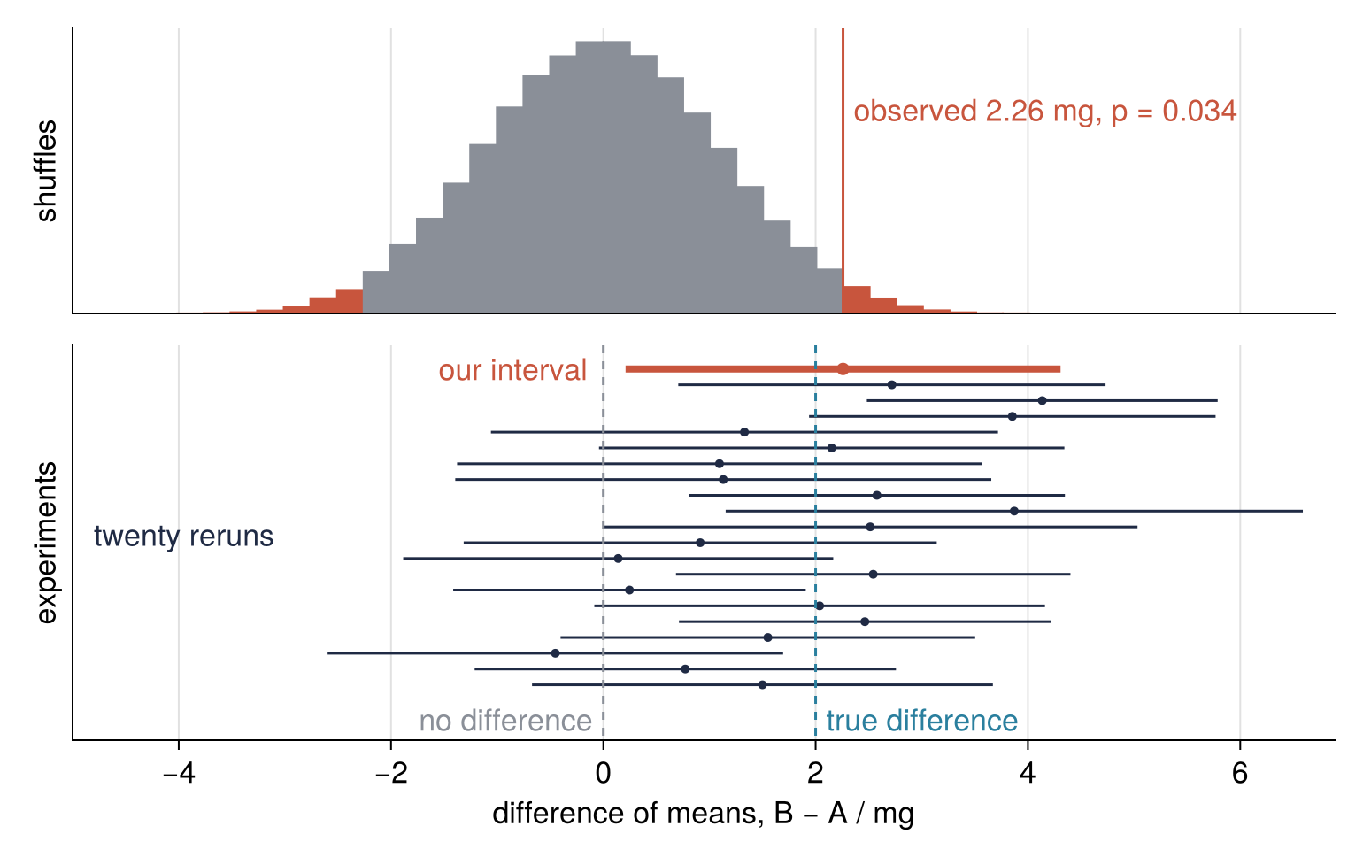
17 of the first twenty intervals catch the true 2.0 mg; just seven stay clear of zero. The other 13 come from experiments run as carefully as ours.

Pitfalls

Believing one p < 0.05 from twelve batches. Repeat an experiment and its p-value lands somewhere else. The reruns of Step 6 measure the spread, and set the runs that pass p < 0.05, the ones a paper calls significant, against all of them:

diffs = [t.xbar for t in tests]
significant = ps .< 0.05
@printf("p over 10,000 reruns: 10th percentile %.3f, 90th percentile %.3f\n", quantile(ps, 0.1), quantile(ps, 0.9))
@printf("mean B − A: all runs %.2f mg, runs with p < 0.05 %.2f mg\n", mean(diffs), mean(diffs[significant]))
@printf("26 batches per protocol: p < 0.05 in %.1f %% of runs\n", 100 * mean(pvalue.(rerun(26)[3]) .< 0.05))

p over 10,000 reruns: 10th percentile 0.003, 90th percentile 0.473
mean B − A: all runs 2.01 mg, runs with p < 0.05 2.82 mg
26 batches per protocol: p < 0.05 in 80.8 % of runs

For one truth, p runs from 0.003 at the 10th percentile to 0.473 at the 90th. With a power under one half, the runs that pass also overestimate the gain: 2.82 mg on average, against 2.01 mg over all runs and the true 2.0 mg. Fix the number of batches before measuring: put your guesses into mu_A, mu_B, and sigma, which rerun reads, and raise n until 80 % of runs pass, the usual target; 26 batches per protocol get this gain past p < 0.05 in 80.8 % of runs. One p = 0.03 from twelve batches justifies a repeat, not a claim.

A t-test on skewed data. Concentrations, grain sizes, and other positive quantities that vary by factors trail off to the right, with a skewness well above zero. The cell takes the 95 % range of skewness for normal samples of twelve from Step 6's reruns. Then it simulates 10,000 experiments with twelve log-normal concentrations per protocol, B's median double A's (LogNormal takes the mean and sd of the logarithm), and counts how often three tests detect the doubling: Welch's on the values, Welch's on their logarithms, and MannWhitneyUTest, which compares ranks, the positions in the sorted pooled sample, instead of means:

s_low, s_high = quantile(skewness.(A), [0.025, 0.975])
R = 10_000
a_ln = [rand(rng, LogNormal(log(10), 1.0), n) for _ in 1:R]     # concentrations, µg/L, median 10
b_ln = [rand(rng, LogNormal(log(20), 1.0), n) for _ in 1:R]     # median 20: B is twice A
skew_ln = skewness.(a_ln)
@printf("normal samples: 95 %% of skewnesses between %.2f and %.2f\n", s_low, s_high)
@printf("log-normal samples: median skewness %.2f, %.0f %% above %.2f\n",
        median(skew_ln), 100 * mean(skew_ln .> s_high), s_high)

found = [
    "t-test on the values"     => pvalue.(UnequalVarianceTTest.(b_ln, a_ln)),
    "t-test on the logarithms" => [pvalue(UnequalVarianceTTest(log.(y), log.(x))) for (x, y) in zip(a_ln, b_ln)],
    "MannWhitneyUTest"         => pvalue.(MannWhitneyUTest.(b_ln, a_ln)),
]
for (name, p) in found
    @printf("%-25s finds the doubling in %.0f %% of pairs\n", name, 100 * mean(p .< 0.05))
end

normal samples: 95 % of skewnesses between -1.09 and 1.13
log-normal samples: median skewness 1.34, 61 % above 1.13
t-test on the values      finds the doubling in 22 % of pairs
t-test on the logarithms  finds the doubling in 36 % of pairs
MannWhitneyUTest          finds the doubling in 33 % of pairs

Among normal samples of twelve, 95 % of skewnesses fall between −1.09 and 1.13, so A's and B's are ordinary. Half the log-normal samples exceed 1.34, yet only 61 % pass 1.13: at twelve values skewness is a weak hint.

A t-test on the raw values detects the doubling in 22 % of the experiments, because means follow the few largest values. On the logarithms, where the ratio becomes a difference, it reaches 36 %, and MannWhitneyUTest 33 %; at twelve values without ties it runs ExactMannWhitneyUTest. So choose by what you know of the quantity, not by the skewness of twelve values: the plain t-test when it varies by amounts, like the yields; the t-test on the logarithms when it varies by factors, like a concentration; MannWhitneyUTest when you cannot say which. The logarithms also give an effect size, a ratio with its interval. Apply exp to the log difference and to both ends of its interval, here for the first experiment:

lr = UnequalVarianceTTest(log.(b_ln[1]), log.(a_ln[1]))
r_low, r_high = exp.(confint(lr))
@printf("B / A = %.2f, 95 %% CI %.2f to %.2f, p = %.3f\n", exp(lr.xbar), r_low, r_high, pvalue(lr))

B / A = 1.41, 95 % CI 0.61 to 3.24, p = 0.403

That is the ratio of geometric means, a geometric mean being the exponentiated mean of the logarithms: B is typically 1.41 times A, between 0.61 and 3.24 times. At p = 0.403 this experiment is a miss. That is the first pitfall again, not a failure of the fix: the interval contains the true ratio of 2.

Reporting significance without an effect size. "Protocol B raised the yield significantly (p = 0.03)" leaves out by how much. A p-value mixes the size of a difference with the number of batches, so with enough batches any difference, however small, drops below 0.05. Report the line from Step 4 instead.

Variations

• Paired measurements. When each specimen is measured before and after a treatment, the samples are linked: OneSampleTTest(after, before) tests the mean of the paired differences.
• Three or more protocols. OneWayANOVATest(a, b, c), an analysis of variance, tests whether any mean differs. HypothesisTests has no Tukey test for which pairs, so run UnequalVarianceTTest per pair and read confint(t; level = 1 - 0.05 / 3), a Bonferroni correction: each of three comparisons gets 0.05 / 3, so together they stay at 0.05.
• A standardized effect size. Cohen's d is the difference in units of the pooled standard deviation, for equal group sizes the root of the mean of both variances. For an interval, bootstrap: redraw each group from itself with sample(rng, x, n; replace = true) from StatsBase, recompute d 10,000 times, and take the quantile at 0.025 and 0.975. The redrawn groups scatter roughly as new experiments would; at twelve values the interval is rough.
• Counts instead of measurements. When you count failed and good batches per protocol, FisherExactTest(failed_A, ok_A, failed_B, ok_B) tests the 2 × 2 table; its confint is for the odds ratio, the odds of failure under A over those under B, 1 for no difference.

Cheat sheet

describe(x); mean(x), std(x), sem(x), skewness(x)         # std and var divide by n − 1
confint(OneSampleTTest(x))                                # 95 % interval of one mean
res = UnequalVarianceTTest(b, a)                          # Welch; the difference is mean(b) − mean(a)
res.xbar, res.stderr, res.t, res.df                       # difference, its standard error, t, effective df
pvalue(res)                                               # two-sided
pvalue(res; tail = :right)                                # one-sided: only if the direction was fixed beforehand
confint(res; level = 0.95)                                # interval of the difference: report this, not p alone
pvalue(ApproximatePermutationTest(rng, b, a, mean, 10^5)) # shuffles, no t distribution
exp.(confint(UnequalVarianceTTest(log.(b), log.(a))))     # skewed positive data: interval of the ratio b / a
pvalue(MannWhitneyUTest(b, a))                            # compares ranks, not means

Further reading

• The HypothesisTests.jl documentation, with the parametric tests (the t-tests) and the nonparametric tests (permutation and Mann-Whitney), and the documentation of StatsBase.jl and Distributions.jl.
• Cumming, Understanding the New Statistics (Routledge, 2012), a book-length case for reporting effect sizes and intervals.
• Wasserstein and Lazar, "The ASA's Statement on p-Values", The American Statistician 70 (2016), the American Statistical Association's own warning against reading p alone.
• On this site: scipy.stats from the ground up: is the difference between two samples real?, the same tutorial in Python, and Fit a curve with error bars and draw a confidence band in Julia.
• Download the notebook. It was executed with the library versions in the header.