Draw a phase portrait of a two-variable ODE system in Julia

The problem

You have a two-variable ODE system and want its phase portrait: one state variable against the other, instead of each against time. Time shows only as motion along a trajectory, the curve one state traces as time runs. The direction field is an arrow at each grid point, pointing where a state there moves next. Fixed points, or steady states, are where both derivatives vanish, so a state there stays. OrdinaryDiffEq, the ODE part of DifferentialEquations.jl, integrates it.

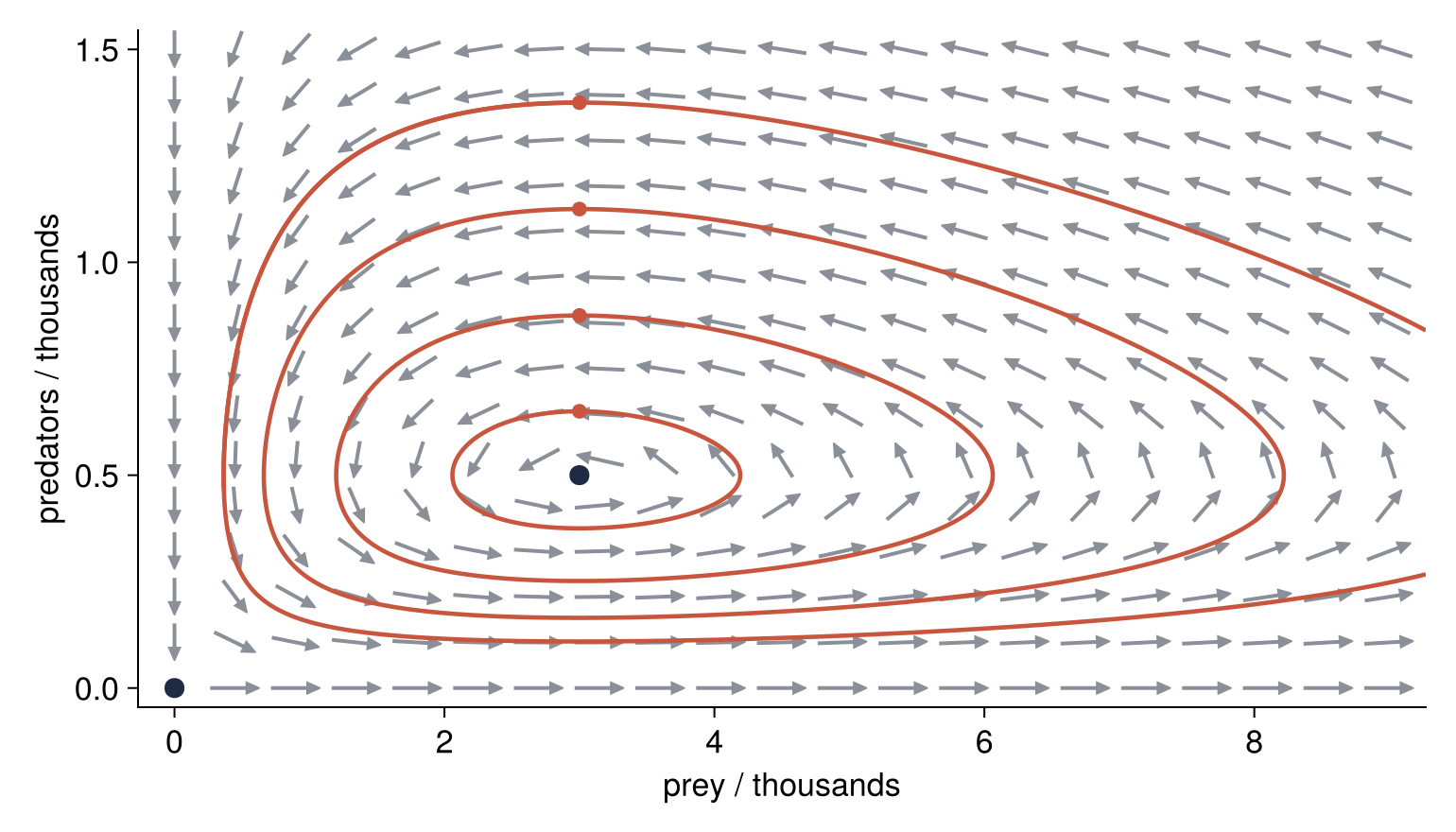
The example is the Lotka-Volterra model of prey \(x\) and predators \(y\), \(\dot x = \alpha x - \beta xy\) and \(\dot y = \delta xy - \gamma y\), with four rates. Swap in your own right-hand side, parameters, window, and starts.

The code

Copy

using OrdinaryDiffEq, NonlinearSolve, Printf, CairoMakie

# ---- system: replace f, its parameters, the window, and the starts with your own
p = (α = 1.0, β = 2.0, γ = 0.6, δ = 0.2)  # a set of named values, read as p.α
# α prey growth, γ predator death: per year; β predation, δ predator gain: per thousand per year
function f(u, p, t)                       # the form ODEProblem calls: state, parameters, time
    x, y = u                              # prey, predators, in thousands
    return [p.α * x - p.β * x * y, p.δ * x * y - p.γ * y]
end
xlim, ylim = (0.0, 9.0), (0.0, 1.5)       # what the figure shows and where the search looks;
inwindow(q) = xlim[1] <= q[1] <= xlim[2] && ylim[1] <= q[2] <= ylim[2]   # the grids follow it
starts = [[3.0, 0.65], [3.0, 0.875], [3.0, 1.125], [3.0, 1.375]]

# ---- direction field
xs, ys = range(xlim[1], xlim[2], length = 21), range(ylim[1], ylim[2], length = 15)
UV = [f([x, y], p, 0.0) for x in xs, y in ys]   # 21 x 15, the whole grid; t does not enter f
U, V = first.(UV), last.(UV)
speed = hypot.(U, V)
L = hypot.(U ./ step(xs), V ./ step(ys))  # in cells (step: one cell); the axes differ in scale
L = ifelse.(L .> 0, L, 1.0)               # a grid point on a fixed point keeps a zero arrow, no 0 / 0
u, v = 0.8 .* U ./ L, 0.8 .* V ./ L       # all 0.8 cells long: raw lengths hide slow regions

# ---- fixed points (steady states): one solve, one zero per guess, so a 5 x 5 grid of guesses
fixed = Vector{Float64}[]
for gx in range(xlim[1], xlim[2], length = 5), gy in range(ylim[1], ylim[2], length = 5)
    # NonlinearProblem wants f(u, p); (u, p) -> ... is an unnamed function that drops t
    sol = solve(NonlinearProblem((u, p) -> f(u, p, 0.0), [gx, gy], p))
    # a failed guess shows in sol.retcode, not as an error; `ok || continue` skips it unless ok
    SciMLBase.successful_retcode(sol) || continue   # SciMLBase comes with NonlinearSolve
    q = round.(sol.u, digits = 6) .+ 0.0  # -1e-15 would print -0.000; adding 0.0 drops the sign
    # keep q if inside (else drawn off the axes) and new (many guesses find the same point)
    inwindow(q) && !any(isapprox(q, r; atol = 1e-6) for r in fixed) && push!(fixed, q)
end

# ---- trajectories
# Tsit5: a standard explicit solver; saveat: report the state every 0.01 years;
# reltol, abstol bound the error of each step (see The knobs); defaults 1e-3, 1e-6
tspan = (0.0, 12.0)                       # years: how far to integrate
trajectories = [solve(ODEProblem(f, u0, tspan, p), Tsit5();
                      saveat = 0.01, reltol = 1e-8, abstol = 1e-10) for u0 in starts]
leaving = count(sol -> !all(inwindow, sol.u), trajectories)   # sol.u: one state per saved time

# ---- report and plot (@printf, @sprintf: C-style formatting from the standard library Printf)
println("fixed points: ", join([@sprintf("(%.3f, %.3f)", q[1], q[2]) for q in fixed], "  "))
@printf("arrow speeds on the grid: %.3g to %.3g\n", minimum(speed[speed .> 0]), maximum(speed))
println("trajectories leaving the window: $leaving of $(length(trajectories))")

fig = Figure(size = (770, 440), fontsize = 17)
ax = Axis(fig[1, 1]; xlabel = "prey / thousands", ylabel = "predators / thousands",
          topspinevisible = false, rightspinevisible = false,
          xgridvisible = false, ygridvisible = false)
arrows2d!(ax, xs, ys, u, v; color = "#8a8f98", align = :center,   # centered on the grid points
          shaftwidth = 2, tiplength = 7, tipwidth = 7)           # pixels; defaults 3, 8, 14
for (sol, u0) in zip(trajectories, starts)
    lines!(ax, first.(sol.u), last.(sol.u); color = "#c8553d", linewidth = 2.3)
    scatter!(ax, u0[1], u0[2]; color = "#c8553d", markersize = 11)
end
scatter!(ax, first.(fixed), last.(fixed); color = "#1f2a44", markersize = 15)
padx, pady = 0.03 * (xlim[2] - xlim[1]), 0.03 * (ylim[2] - ylim[1])   # room for the corner marker
limits!(ax, xlim[1] - padx, xlim[2] + padx, ylim[1] - pady, ylim[2] + pady)   # last: frame = window
fig

fixed points: (0.000, 0.000)  (3.000, 0.500)
arrow speeds on the grid: 0.0643 to 18.1
trajectories leaving the window: 1 of 4

The knobs

The 21 × 15 grid puts about twenty arrows across, enough to follow the flow. arrows2d! draws each vector in data units, so on a window 9 wide and 1.5 high a unit vector pointing up comes out about three times longer on screen than one pointing across; normalize = true works in data units too. Lengths in grid cells keep every direction and come out equal; 0.8 of a cell leaves a gap. The 5 × 5 guesses span the window, so a fixed point outside it is never found: give the window a margin. The starts sit on a vertical line through \((3, 0.5)\), so the closed trajectories nest. If your trajectories run into a fixed point instead of circling, start a few states just off each fixed point, to see which ones attract, and a few along the window edge, to see where distant states go. tspan is the setting to lengthen: 12 years lets the widest trajectory close, a trajectory that ends in midair has run out of time, and saveat follows the span by itself. The solver shrinks each step until its estimated error is below abstol + reltol * abs(u), so reltol sets the correct digits, about eight here, and abstol, in state units, goes well below the smallest value that matters, as 1e-10 does below predators of order 0.1. The DifferentialEquations.jl accuracy step has the rest.

Of equal length, an arrow tells which way a state at its center moves and not how fast. Color brings speed back: add color = vec(speed), colormap = :cividis to arrows2d!, vec flattening the matrix in arrow order. \((0, 0)\) is extinction, since each derivative carries a factor of its own variable. Away from the axes, setting both right-hand sides to zero leaves \(y = \alpha/\beta\) and \(x = \gamma/\delta\), which is \((3, 0.5)\): NonlinearSolve matches the hand solution. The dark markers only show where f is zero; the trajectories show whether states approach them. They loop around \((3, 0.5)\) and never get there, and at the origin states come in down the predator axis and go out along the prey axis. All of this needs an f without \(t\) in it, so each point keeps one arrow. Under a periodic input, such as a cycled temperature, record the state once per period instead, a Poincaré section, as in the DifferentialEquations.jl variations.

Pitfalls

Arrows scaled by speed. Hand U, V to arrows2d! instead of u, v, and each arrow is drawn at its raw length in data units. In the upper right they run up to 18 units, twice the width of the window, and pile into a tangle, while around \((3, 0.5)\) they shrink to bare arrowheads. The second printed line gives the range, 0.0643 to 18.1 thousand per year, a factor of 281, and Makie applies no common scale at all. Yet every fixed point lies where the flow is slow, so the arrows you lose are the ones the portrait is for. Give every arrow the same length, as the code does.

Trajectories that run past the window. One of the four, the outermost, crosses the right edge and returns, as the last printed line reports. Delete the limits! line and Makie widens the axes to fit every point plotted, that trajectory included, while the arrows stop short of the new edge. For a system that runs away, also stop the integration with a condition that changes sign at the edge of a box larger than the window, such as box(u, t, integrator) = min(u[1] + 1, 20 - u[1], u[2] + 1, 5 - u[2]). Pass callback = ContinuousCallback(box, terminate!) to solve, and the solver stops where box crosses zero. The ContinuousCallback step of the DifferentialEquations.jl tutorial covers callbacks in full.

Too many arrows. On a 60 × 60 grid the arrows merge into a gray texture. Draw lines instead, with streamplot!(ax, (x, y) -> Point2f(f([x, y], p, 0.0)), xlim[1]..xlim[2], ylim[1]..ylim[2]; color = _ -> "#8a8f98"). Point2f is Makie's type for a point of two numbers, which streamplot wants back from the function; a..b is the closed interval from a to b, available after using CairoMakie; _ -> "#8a8f98" ignores its argument, because color must be a function and by default colors by speed. Its lines are steps of a fixed 0.01 along the direction of f, without the error control the tolerances give solve, so they show the flow but solve nothing to a tolerance.