The adjoint method: why 200 derivatives cost two solves, not 201

The question

A drill core of layered sediment, 1 m long, lies on a bench. A heater pushes 100 W/m² into its left end, the right end sits in a 20 °C bath, and once the core has settled, which for a meter of rock takes weeks, twenty thermometers 5 cm apart read from 65.66 °C at the heater down to 21.90 °C at 0.95 m. You want the conductivity along the core, 200 conductivities for 200 cells of 5 mm, and you will fit them by following the gradient of the misfit. The adjoint method is what makes that gradient cheap.

The model is the steady heat equation on those cells. Each cell is a thermal resistor \(\Delta x/k_i\) between the nodes at its two ends, so the node temperatures \(u\) solve \(K(k)\,u = f\), the Kirchhoff system of the resistor network with temperature for voltage and heat flux for current. \(K\) is tridiagonal, symmetric, and linear in \(k\); \(f\) holds the heater flux at the first node and the bath at the last.

import numpy as np
import matplotlib.pyplot as plt
from scipy import sparse
from scipy.sparse.linalg import spsolve, factorized
from scipy.optimize import minimize, minimize_scalar, brentq

plt.rcParams.update({
    "figure.figsize": (8, 3.2), "figure.dpi": 110,
    "axes.spines.top": False, "axes.spines.right": False,
    "axes.grid": True, "grid.alpha": 0.25,
    "font.size": 11, "lines.linewidth": 1.8,
})
INK, ACCENT, SECOND, MUTED = "#1f2a44", "#c8553d", "#2a7f9e", "#8a8f98"

n, dx = 200, 0.005                         # cells, cell length / m
q, T_R, sigma = 100.0, 20.0, 0.02          # heater / (W/m²), bath / °C, noise / K
x = np.arange(n + 1) * dx                  # nodes at the cell boundaries; node n is the bath
sensors = np.arange(0, n, 10)              # thermometers at 0, 0.05, ..., 0.95 m
P = sparse.csr_array((np.ones(sensors.size), (np.arange(sensors.size), sensors)), shape=(sensors.size, n))

# The core is synthetic, so the answer can be checked at the end. Pretend you have not seen these layers.
edges = np.array([0, 0.12, 0.27, 0.35, 0.52, 0.60, 0.78, 0.86, 1.0])
k_layer = np.array([2.8, 1.6, 3.6, 2.2, 1.2, 3.0, 2.0, 2.6])               # W/(m K)
k_true = k_layer[np.searchsorted(edges, x[:-1] + dx / 2, side="right") - 1]

def K_of(k):
    c = k / dx                             # conductance of each cell
    main = c.copy()
    main[1:] += c[:-1]
    return sparse.diags_array([main, -c[:-1], -c[:-1]], offsets=[0, 1, -1], format="csc")

def rhs(k):
    f = np.zeros(n)
    f[0] = q                               # the heater
    f[-1] = k[-1] / dx * T_R               # the bath, through the last cell
    return f

def forward(k):
    return spsolve(K_of(k), rhs(k))

def misfit(k):
    return 0.5 * np.sum(((forward(k)[sensors] - d) / sigma) ** 2)

rng = np.random.default_rng(7)
u_true = forward(k_true)
closed_form = T_R + q * np.cumsum((dx / k_true)[::-1])[::-1]
d = u_true[sensors] + sigma * rng.standard_normal(sensors.size)
print(f"model against closed form: {np.abs(u_true - closed_form).max():.0e} K")

model against closed form: 7e-14 K

Show code

Copy

k0 = minimize_scalar(lambda c: misfit(np.full(n, c)), bounds=(0.5, 5), method="bounded").x
k_start = np.full(n, k0)
u0 = forward(k_start)
print(f"best uniform rod: k = {k0:.2f} W/(m K), largest miss {np.abs(u0[sensors] - d).max():.2f} K")

fig, ax = plt.subplots()
ax.plot(x, np.append(u0, T_R), color=MUTED, lw=1.6)        # the starting guess, context
ax.plot(x[sensors], d, "o", color=INK, ms=5)
ax.text(0.45, 52, f"uniform rod, k = {k0:.2f} W/(m K)", color=MUTED)
worst = np.abs(u0[sensors] - d).argmax()                # the largest miss, as a bracket
xw = x[sensors][worst]
ax.plot([xw, xw], [d[worst], u0[sensors][worst]], color=MUTED, lw=1.2, zorder=0)
ax.annotate(f"largest miss {np.abs(u0[sensors] - d).max():.2f} K", (xw, (d[worst] + u0[sensors][worst]) / 2),
            xytext=(0.3, 28), color=MUTED, arrowprops=dict(arrowstyle="-", color=MUTED, lw=1))
ax.set(xlabel="x / m", ylabel="temperature / °C", xlim=(0, 1))
plt.show()

best uniform rod: k = 2.21 W/(m K), largest miss 2.72 K

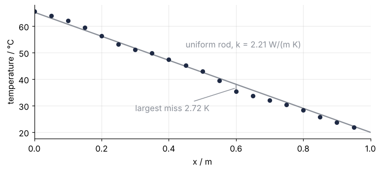
Two things are obvious. The core is not uniform: the best single conductivity, 2.21 W/(m K), misses the readings by up to 2.72 K, a hundred times the thermometers' noise of 0.02 K. And the way to find 200 conductivities is to walk downhill on the misfit \(J = \tfrac12\sum_s \big((T_s - d_s)/\sigma\big)^2\), half the sum of the squared misses of the model temperatures \(T_s\) against the readings \(d_s\), in units of the noise \(\sigma\). That is gradient descent, and it needs the slope in 200 directions at every step. The slope of \(J\) against one model temperature, \(\tilde r_s = (T_s - d_s)/\sigma^2\), is the weighted residual of that thermometer.

The direct way to get that slope nudges one cell, solves again, and repeats: 201 solves per gradient with one-sided differences, 401 with central ones, and the fit needs a few hundred gradients. Less obvious: all 200 derivatives come from one extra solve, whatever the number of cells.

The idea: ask the thermometers, not the cells

Raise the conductivity of one cell by 1 % and solve again. In steady conduction along a rod the change is a step: the same 100 W/m² now passes a slightly smaller resistance, so every node between the heater and that cell drops by the same small amount, and nothing downstream moves. The misfit changes by that drop times the sum of the weighted residuals of the upstream thermometers. Here are three cells, at 0.2, 0.5, and 0.8 m, on the uniform rod of 2.21 W/(m K), where the fit takes its first step and every figure up to the gradient check is drawn.

Show code

Copy

r0 = u0[sensors] - d                                    # model minus data / K
cells = [40, 100, 160]
dJ_brute = []
fig, axes = plt.subplots(3, 1, figsize=(8, 6.5), sharex=True)
for ax, i in zip(axes, cells):
    k = k_start.copy()
    k[i] *= 1.01
    du = np.append(forward(k) - u0, 0.0)
    dJ_brute.append(misfit(k) - misfit(k_start))
    ax.axvspan(x[i], x[i + 1], color=MUTED, alpha=0.4, lw=0)
    ax.plot(x, 1e3 * du, color=SECOND)                  # a brute-force re-solve
    warm = r0 > 0
    ax.plot(x[sensors][warm], 1e3 * du[sensors][warm], "o", color=SECOND, ms=5)
    ax.plot(x[sensors][~warm], 1e3 * du[sensors][~warm], "o", mfc="white", color=SECOND, ms=5)
    label = f"cell at {x[i]:.2f} m   δJ = {dJ_brute[-1]:+.1f}".replace("-", "−")
    right = x[i] < 0.6                                  # on the wider side of the step
    ax.text(0.99 if right else 0.01, -1.2, label, transform=ax.get_yaxis_transform(), ha="right" if right else "left")
    ax.set(ylabel="δT / mK", ylim=(-2.8, 0.6))
axes[-1].set(xlabel="x / m", xlim=(0, 1))
plt.show()
print(f"drop upstream of the cell: {1e3 * (forward(k) - u0)[0]:.2f} mK")

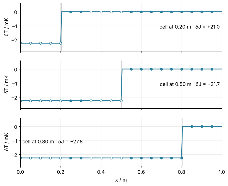
drop upstream of the cell: -2.24 mK

Filled dots are thermometers where the uniform rod reads too warm, open ones where it reads too cool. Cooling the five thermometers up to 0.2 m raises the misfit by 21.0, because they read too cool on balance; cooling the seventeen up to 0.8 m lowers it by 27.8. Each number cost a solve, and there are 200 cells.

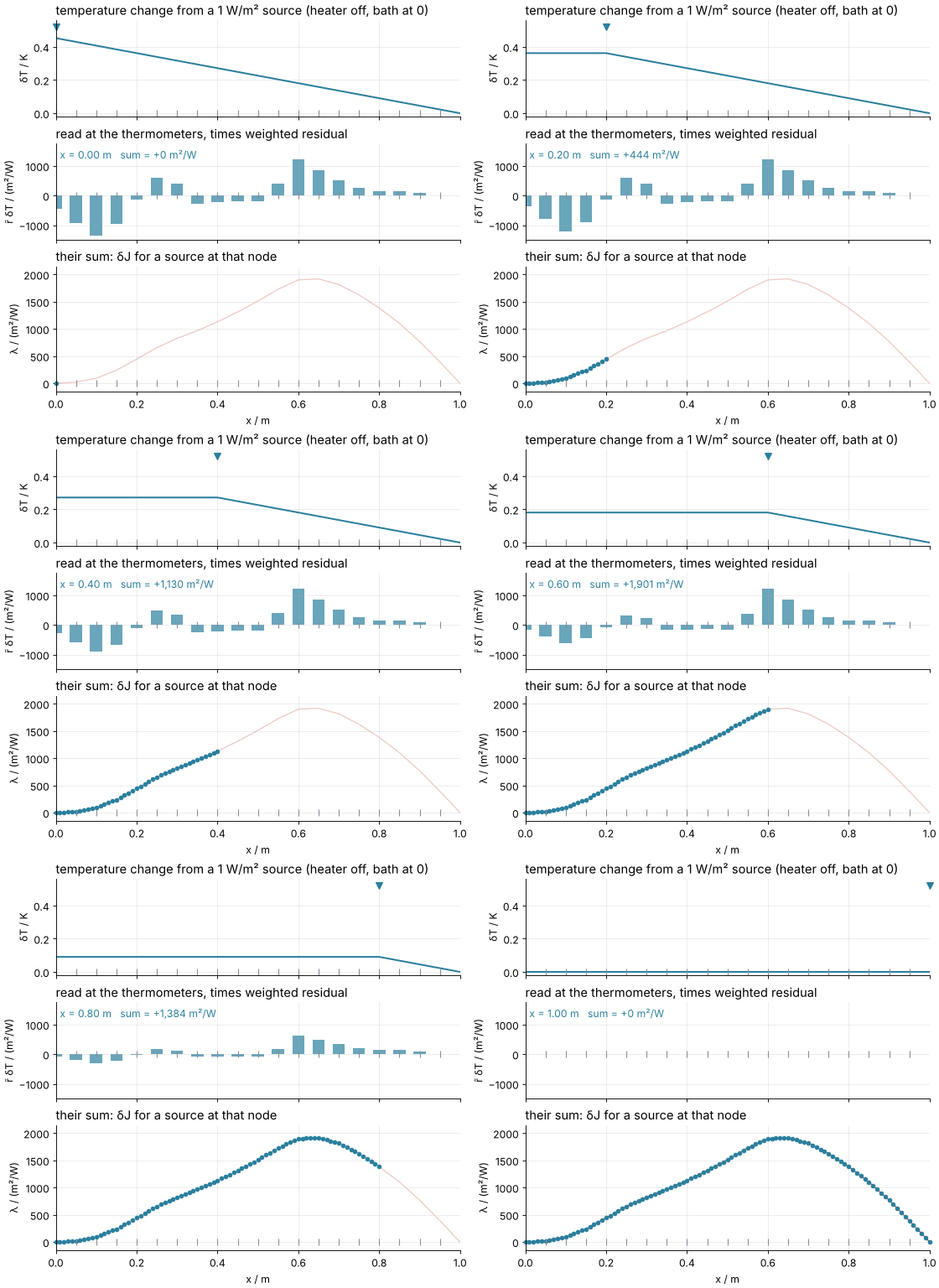
Now turn it around. A change in one cell acts on the temperatures like a pair of heat sources of opposite sign at its two nodes (the next section gives their strength). So what you need is how the misfit answers a small heat source at each node, the field \(\lambda_j = \partial J/\partial f_j\). That looks like 200 more solves, but reciprocity says otherwise: the temperature at a thermometer due to a source at node \(j\) equals the temperature at node \(j\) due to the same source at the thermometer, because \(K\) is symmetric and so is \(K^{-1}\). All 200 answers therefore come from one solve. Put a heat source at each thermometer, of strength equal to its weighted residual \(\tilde r_s\), and the temperature it makes is \(\lambda\).

Where the model reads too warm, more heat would make things worse, so that thermometer is a source and \(\lambda\) rises around it; where it reads too cool, the thermometer is a sink. These sources heat a second, imagined copy of the core, the adjoint problem, and its ends follow from what an added source changes. The heater flux stays 100 W/m² and the bath stays 20 °C whatever you add, so the change at both ends is zero: in the copy the heater is off and the bath is at 0 °C. No flux enters \(\lambda\) at the left end except what the thermometer at \(x = 0\) puts in, and \(\lambda\) is zero at the bath.

r_w = r0 / sigma**2                                     # weighted residuals / K⁻¹
lam = spsolve(K_of(k_start).T, P.T @ r_w)               # the one adjoint solve
lam_brute = [r_w @ spsolve(K_of(k_start), np.eye(n)[j])[sensors] for j in sensors]

print(f"residuals: {r0.min():+.2f} K at {x[sensors][r0.argmin()]:.2f} m to {r0.max():+.2f} K at {x[sensors][r0.argmax()]:.2f} m")
print("signs from 0 to 0.95 m:  " + " ".join("+" if r > 0 else "−" for r in r0))
print(f"λ: {lam[0]:+.3f} m²/W at x = 0, largest {lam.max():,.0f} m²/W at {x[lam.argmax()]:.2f} m, "
      f"{lam[sensors[-1]]:,.0f} m²/W at the last thermometer")
print(f"adjoint against one source per thermometer node: largest gap {np.abs(lam[sensors] - lam_brute).max():.0e} m²/W")

residuals: -1.34 K at 0.10 m to +2.72 K at 0.60 m
signs from 0 to 0.95 m:  − − − − − + + − − − − + + + + + + + + +
λ: -0.060 m²/W at x = 0, largest 1,920 m²/W at 0.65 m, 395 m²/W at the last thermometer
adjoint against one source per thermometer node: largest gap 2e-12 m²/W

On the uniform rod the residuals run from −1.34 K at 0.10 m to +2.72 K at 0.60 m, and the signs alternate: too cool up to 0.20 m, too warm at 0.25 and 0.30 m, too cool again from 0.35 to 0.50 m, and too warm from 0.55 m to the end. \(\lambda\) is −0.060 m²/W at the heater, positive everywhere else, largest at 0.65 m with 1,920 m²/W, and down to 395 m²/W at the last thermometer. Twenty brute-force solves, a unit source at each thermometer node, agree with it to rounding. Done at every node, the brute force traces the whole curve:

"""Source sweep: lambda traced point by point by brute force, and found by one adjoint solve.

Renders ../../assets/source-sweep.gif. The core, its data, and the uniform start are those
of the tutorial py-adjoint-method. Run it from any directory:

    python scene.py
"""
from pathlib import Path

import numpy as np
import matplotlib.pyplot as plt
from matplotlib.animation import FuncAnimation, PillowWriter
from scipy import sparse
from scipy.sparse.linalg import spsolve
from scipy.optimize import minimize_scalar

OUT = Path(__file__).resolve().parents[2] / "assets" / "source-sweep.gif"
ACCENT, SECOND, MUTED = "#c8553d", "#2a7f9e", "#8a8f98"
plt.rcParams.update({"axes.spines.top": False, "axes.spines.right": False,
                     "axes.grid": True, "grid.alpha": 0.25, "font.size": 11})

# ---- the core of the tutorial, its readings, and the best uniform rod
n, dx, q, T_R, sigma = 200, 0.005, 100.0, 20.0, 0.02
edges = np.array([0, 0.12, 0.27, 0.35, 0.52, 0.60, 0.78, 0.86, 1.0])
k_layer = np.array([2.8, 1.6, 3.6, 2.2, 1.2, 3.0, 2.0, 2.6])
x = np.arange(n + 1) * dx
k_true = k_layer[np.searchsorted(edges, x[:-1] + dx / 2, side="right") - 1]
sensors = np.arange(0, n, 10)

def K_of(k):
    c = k / dx
    main = c.copy()
    main[1:] += c[:-1]
    return sparse.diags_array([main, -c[:-1], -c[:-1]], offsets=[0, 1, -1], format="csc")

def forward(k):
    f = np.zeros(n)
    f[0], f[-1] = q, k[-1] / dx * T_R
    return spsolve(K_of(k), f)

rng = np.random.default_rng(7)
d = forward(k_true)[sensors] + sigma * rng.standard_normal(sensors.size)
k0 = minimize_scalar(lambda c: np.sum((forward(np.full(n, c))[sensors] - d) ** 2),
                     bounds=(0.5, 5), method="bounded").x
K = K_of(np.full(n, k0))
r_w = (forward(np.full(n, k0))[sensors] - d) / sigma**2               # weighted residuals / K⁻¹
lam = np.append(spsolve(K.T, np.bincount(sensors, r_w, n)), 0.0)      # one adjoint solve; bath node 0

# ---- the brute-force sweep: a unit source at node j, heater off, bath at 0
frames = np.arange(0, n + 1, 2)

def response(j):
    if j == n:                                                        # a source in the bath does nothing
        return np.zeros(n + 1)
    e = np.zeros(n)
    e[j] = 1.0
    return np.append(spsolve(K, e), 0.0)

sweep = {j: response(j) for j in frames}
traced = {j: r_w @ sweep[j][sensors] for j in frames}

# ---- figure, drawn once
fig, (ax1, ax2, ax3) = plt.subplots(3, 1, figsize=(7, 6.4), dpi=80, sharex=True,
                                    height_ratios=[1, 1, 1.3], layout="constrained")
# the brute force in SECOND throughout; ACCENT is λ from the adjoint solve
(du_line,) = ax1.plot([], [], color=SECOND, lw=1.8)
(src,) = ax1.plot([], [], "v", color=SECOND, ms=8, clip_on=False)               # marks the source node
bars = ax2.bar(x[sensors], np.zeros(sensors.size), width=0.03, color=SECOND, alpha=0.7)
sum_text = ax2.text(0.01, 0.95, "", transform=ax2.transAxes, ha="left", va="top", color=SECOND)
lam_faint = ax3.plot(x, lam, color=ACCENT, lw=1.2, alpha=0.3)[0]
(dots,) = ax3.plot([], [], "o", color=SECOND, ms=4, clip_on=False)
for ax in (ax1, ax2, ax3):
    ax.plot(x[sensors], np.zeros(sensors.size), "|", color=MUTED, ms=8)
ax1.set(ylabel="δT / K", ylim=(-0.02, 0.56))
ax2.set(ylabel="r̃ δT / (m²/W)", ylim=(-1500, 1750))
ax3.set(ylabel="λ / (m²/W)", xlabel="x / m", xlim=(0, 1), ylim=(-150, 2150))
ax1.set_title("temperature change from a 1 W/m² source (heater off, bath at 0)", loc="left")
ax2.set_title("read at the thermometers, times weighted residual", loc="left")
ax3.set_title("their sum: δJ for a source at that node", loc="left")

def update(j):
    du = sweep[j]
    du_line.set_data(x, du)
    src.set_data([x[j]], [0.52])
    for bar, h in zip(bars, r_w * du[sensors]):
        bar.set_height(h)
    sum_text.set_text(f"x = {x[j]:.2f} m   sum = {round(traced[j]):+,d} m²/W".replace("-", "−"))
    shown = frames[frames <= j]
    dots.set_data(x[shown], [traced[s] for s in shown])
    lam_faint.set_alpha(1.0 if j == frames[-1] else 0.3)

OUT.parent.mkdir(exist_ok=True)
FuncAnimation(fig, update, frames=list(frames) + [frames[-1]] * 12).save(OUT, writer=PillowWriter(fps=12))
plt.close(fig)
print(f"{OUT.name}: {OUT.stat().st_size / 1024:,.0f} kB, largest brute-force/adjoint gap "
      f"{max(abs(traced[j] - lam[j]) for j in frames):.1e} m²/W")

From a heat source to a conductivity

Raising \(k_i\) by \(\delta k\) lets more heat through cell \(i\) at the old temperatures, \(\delta k\,(u_i - u_{i+1})/\Delta x\) more. That heat leaves node \(i\) and arrives at node \(i+1\): a sink at \(i\) and a source at \(i+1\) of that strength. For a 1 % change it is 1 % of the flux through the cell, which in this rod is always \(q\), so 1 W/m² at every cell. Each source changes \(J\) by its strength times \(\lambda\) at its node, and the two together give

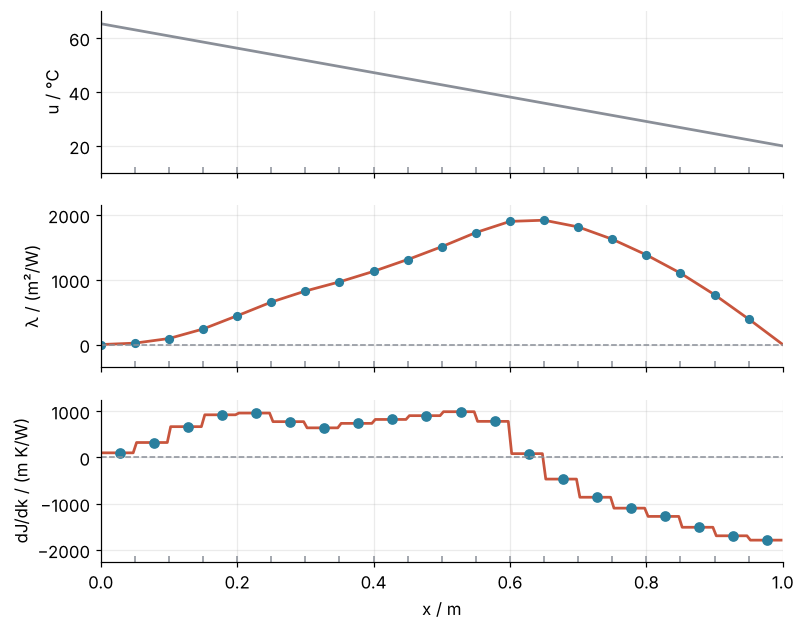
the drop of \(\lambda\) across the cell times the drop of the temperature, one product per cell. For the three cells of the step figure, −1 W/m² times the drop of \(\lambda\) predicts the change of the misfit:

Show code

Copy

u_e, lam_e = np.append(u0, T_R), np.append(lam, 0.0)   # the bath node: u = T_R, λ = 0
grad = -(lam_e[:-1] - lam_e[1:]) * (u_e[:-1] - u_e[1:]) / dx
for i, dJ in zip(cells, dJ_brute):
    print(f"cell at {x[i]:.2f} m:  δJ = {dJ:+6.1f}   predicted {-(lam_e[i] - lam_e[i + 1]):+6.1f}")

h = 1e-4
check = np.arange(5, n, 10)
grad_fd = [(misfit(k_start + h * np.eye(n)[i]) - misfit(k_start - h * np.eye(n)[i])) / (2 * h) for i in check]

fig, (ax1, ax2, ax3) = plt.subplots(3, 1, figsize=(8, 6.5), sharex=True)
ax1.plot(x, u_e, color=MUTED)                          # the uniform start, as in the first figure
ax1.set(ylabel="u / °C", ylim=(10, 70))
ax2.plot(x, lam_e, color=ACCENT)
ax2.plot(x[sensors], lam_brute, "o", color=SECOND, ms=5)
ax2.axhline(0, color=MUTED, lw=1, ls="--")
ax2.set(ylabel="λ / (m²/W)", ylim=(-350, 2150))
ax3.plot(x[:-1] + dx / 2, grad, color=ACCENT)
ax3.plot(x[check] + dx / 2, grad_fd, "o", color=SECOND, ms=6)
ax3.axhline(0, color=MUTED, lw=1, ls="--")
ax3.set(xlabel="x / m", ylabel="dJ/dk / (m K/W)", xlim=(0, 1), ylim=(-2250, 1250))
for ax in (ax1, ax2, ax3):                              # the thermometers, on the x axis
    ax.plot(x[sensors], np.zeros(sensors.size), "|", color=MUTED, ms=8, transform=ax.get_xaxis_transform())
plt.show()

print("dJ/dk per 5 cm segment / (m K/W):")
print(np.array2string(grad[::10], precision=0, separator=", ", max_line_width=90, floatmode="fixed"))

cell at 0.20 m:  δJ =  +21.0   predicted  +21.2
cell at 0.50 m:  δJ =  +21.7   predicted  +21.8
cell at 0.80 m:  δJ =  -27.8   predicted  -28.2

dJ/dk per 5 cm segment / (m K/W):
[   99.,   322.,   665.,   921.,   959.,   774.,   639.,   736.,   821.,   903.,   988.,
   780.,    82.,  -468.,  -861., -1096., -1275., -1509., -1694., -1788.]

The prediction is off by about 1 %, the second-order part of a 1 % change, which a derivative leaves out. \(\lambda\) is the curve the animation traced, with the ends of the adjoint problem. Central differences at every tenth cell sit on the adjoint gradient.

The adjoint flux through a cell, \(k_i(\lambda_i - \lambda_{i+1})/\Delta x\), is the sum of the weighted residuals of all thermometers upstream, since the left end lets none in. On a uniform rod the slope of \(\lambda\) is that flux divided by the one \(k\): \(\lambda\) climbs where the upstream thermometers read too cool on balance, falls where they read too warm, and runs straight between thermometers. Since every cell carries the same \(q\), \(u_i - u_{i+1} = q\,\Delta x/k_i\), and the gradient is minus the adjoint flux times \(q\,\Delta x/k_i^2\). At the uniform start it is therefore constant in each segment, from +988 m K/W at 0.50 to 0.55 m, where the upstream thermometers read too cool on balance, to −1,788 m K/W in the last segment, where all twenty residuals add up too warm and raising \(k\) cools them.