Finite differences: the heat equation as a matrix, and why the time step has a limit

The question

A copper rod 1 m long sits at 0 °C. At \(t = 0\) its left end is put to 100 °C, the right end is held at 0 °C, and within about an hour the temperature settles to a straight line between the two. To compute this with finite differences, cut the rod into 50 pieces of 2 cm and replace the heat equation, \(\partial T/\partial t = D\,\partial^2 T/\partial x^2\), by one rule per grid point: in each time step a point's temperature moves toward the mean of its two neighbors. The diffusivity \(D\) = 1.17 × 10⁻⁴ m²/s is that of pure copper at 300 K, from Incropera's Fundamentals of Heat and Mass Transfer, Table A.1. Here it is with steps of 1.5 s and of 3.0 s:

Show code

Copy

import numpy as np
import matplotlib.pyplot as plt

plt.rcParams.update({
    "figure.figsize": (8, 3.4), "figure.dpi": 110,
    "axes.spines.top": False, "axes.spines.right": False,
    "axes.grid": True, "grid.alpha": 0.25,
    "font.size": 11, "lines.linewidth": 1.8,
})
INK, ACCENT, SECOND, MUTED = "#1f2a44", "#c8553d", "#2a7f9e", "#8a8f98"

L, D = 1.0, 1.17e-4                   # m, m²/s (copper at 300 K)
n = 50                                # pieces; 51 grid points, 49 of them unknown
dx = L / n
x = np.linspace(0, L, n + 1)
T_hot = 100.0                         # °C at x = 0; the right end stays at 0 °C
m = n - 1

# second difference of the 49 interior points, and the hot end's contribution
A = (np.diag(np.full(m, -2.0)) + np.diag(np.ones(m - 1), 1) + np.diag(np.ones(m - 1), -1)) / dx**2
b = np.zeros(m)
b[0] = T_hot / dx**2
T_line = T_hot * (1 - x / L)          # the steady state, a straight line


def run(dt, n_steps, keep=()):
    """Explicit steps from the cold rod; returns the full profiles (ends included) at the steps in keep."""
    T = np.zeros(m)
    kept = {}
    for step in range(1, n_steps + 1):
        T = T + dt * D * (A @ T + b)
        if step in keep:
            kept[step] = np.concatenate([[T_hot], T, [0.0]])
    return kept


stable = run(1.5, 2400, keep={40, 200, 800, 2400})
unstable = run(3.0, 10, keep={3, 5, 10})

for step, T in stable.items():
    print(f"dt = 1.5 s, t = {step * 1.5 / 60:4.0f} min: max |T - line| = {np.abs(T - T_line).max():6.2f} °C")
for step, T in unstable.items():
    print(f"dt = 3.0 s, step {step:2d}:      max |T| = {np.abs(T).max():9,.0f} °C")

fig, (ax0, ax1) = plt.subplots(1, 2, sharey=True)
for ax in (ax0, ax1):
    ax.plot(x, T_line, color=INK, lw=1)
    ax.set(xlabel="x / m", xlim=(0, L))
for (step, T), alpha in zip(stable.items(), [0.35, 0.55, 0.75, 1.0]):
    ax0.plot(x, T, color=ACCENT, alpha=alpha, label=f"{step * 1.5 / 60:.0f} min")
ax0.legend(frameon=False, loc="lower right", ncols=2, handlelength=1.4, columnspacing=1.2,
           labelspacing=0.3, borderaxespad=0.2)
ax0.text(0.97, 0.95, "Δt = 1.5 s", transform=ax0.transAxes, ha="right", va="top", color=ACCENT)
T10 = unstable[10]
ax1.plot(x, T10, "o-", color=SECOND, ms=3, lw=1)
ax1.text(0.97, 0.95, f"Δt = 3.0 s, after 10 steps\nmax |T| = {np.abs(T10).max():,.0f} °C",
         transform=ax1.transAxes, ha="right", va="top", color=SECOND)
ax0.set(ylabel="T / °C", ylim=(-50, 150))
plt.show()

dt = 1.5 s, t =    1 min: max |T - line| =  71.71 °C
dt = 1.5 s, t =    5 min: max |T - line| =  46.86 °C
dt = 1.5 s, t =   20 min: max |T - line| =  15.91 °C
dt = 1.5 s, t =   60 min: max |T - line| =   0.99 °C
dt = 3.0 s, step  3:      max |T| =       139 °C
dt = 3.0 s, step  5:      max |T| =       312 °C
dt = 3.0 s, step 10:      max |T| =    16,708 °C

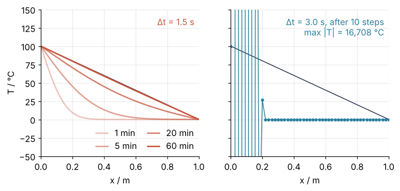
The left panel is what you expect. After 1 min the warmth has reached about 20 cm into the rod, after 20 min it is still 15.91 °C away from the line at its worst, and after 60 min and 2,400 steps no point is more than 0.99 °C from it. The right panel doubles the step and stops after ten steps, 30 s of rod time. At step 3 a point near the hot end is at 139 °C, on a rod whose ends are at 0 and 100 °C. At step 10 neighbors alternate in sign, the largest magnitude is 16,708 °C, and the sawtooth covers exactly the first 20 cm: ten pieces in ten steps.

The obvious lesson is that a smaller step is more accurate. It is not the lesson here: halving the step from 3.0 to 1.5 s does not improve a result, it turns nonsense into an answer. Somewhere between the two lies a sharp threshold. Why is there one, why at the value it has, why does the failure look like a sawtooth, and why does it not care how hot the rod is or how long you run?

The idea: each piece moves toward the average of its neighbors

Fourier's law says heat flows between two touching pieces in proportion to their temperature difference. Piece \(j\) gains from its left neighbor in proportion to \(T_{j-1} - T_j\) and from its right neighbor in proportion to \(T_{j+1} - T_j\). Add the two and the net gain is proportional to \(T_{j-1} - 2T_j + T_{j+1}\), which is twice the distance from \(T_j\) to the mean of its neighbors. A piece colder than that mean warms, a warmer one cools, and on a straight line every piece already sits at the mean of its neighbors. That is why the rod ends up straight.

Over one time step \(\Delta t\) this is the update

The number \(2r\) is the fraction of the way to its neighbors' mean that a piece covers in one step. \(D/\Delta x^2\) is a rate, 0.29 per second for this rod, and the step decides how much of it is taken at once. Here is the very first step at the hot end, for three step sizes:

Show code

Copy

print(f"D / dx² = {D / dx**2:.2f} per second")
T0 = np.concatenate([[T_hot], np.zeros(m), [0.0]])
fig, axes = plt.subplots(1, 3, figsize=(8, 2.8), sharey=True)
for ax, dt in zip(axes, [0.75, 1.5, 3.0]):
    r = D * dt / dx**2
    T1 = run(dt, 1, keep={1})[1]
    color = ACCENT if r <= 0.5 else SECOND
    print(f"dt = {dt:4.2f} s, r = {r:.3f}: first point {T1[1]:5.1f} °C, "
          f"neighbors' mean {(T0[0] + T0[2]) / 2:.0f} °C, second point {T1[2]:.1f} °C")
    ax.plot([x[1] - 0.006, x[1] + 0.006], [50, 50], color=MUTED, ls="--", lw=1)
    ax.plot(x[:6], T1[:6], "o", color=color, ms=6)
    ax.plot(x[:6], T0[:6], "o", color=MUTED, ms=10, mfc="none", mew=1.2)   # before: rings
    ax.annotate("", (x[1], T1[1]), (x[1], 0), arrowprops=dict(arrowstyle="->", color=color, lw=1.2))
    ax.text(x[1] + 0.008, T1[1], f"{T1[1]:.1f} °C", color=color, va="center")
    ax.text(0.03, 0.97, f"Δt = {dt} s, r = {r:.3f}", transform=ax.transAxes, va="top", color=color)
    ax.set(xlabel="x / m", xlim=(-0.005, 0.105), ylim=(-8, 132))
axes[0].text(x[1] + 0.008, 50, "neighbors' mean", color=MUTED, va="center")
axes[0].set_ylabel("T / °C")
plt.show()

D / dx² = 0.29 per second
dt = 0.75 s, r = 0.219: first point  21.9 °C, neighbors' mean 50 °C, second point 0.0 °C
dt = 1.50 s, r = 0.439: first point  43.9 °C, neighbors' mean 50 °C, second point 0.0 °C
dt = 3.00 s, r = 0.877: first point  87.7 °C, neighbors' mean 50 °C, second point 0.0 °C

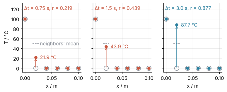
The first interior point has neighbors at 100 and 0 °C, so their mean is 50 °C. With \(\Delta t\) = 0.75 s it covers \(2r\) = 44 % of the way and lands at 21.9 °C, with 1.5 s it reaches 43.9 °C, still short. With 3.0 s the panel's \(r\) = 0.877 doubles to \(2r\) = 1.75: the point covers 175 % of the way and lands at 87.7 °C, beyond the mean. The second point stays at 0 °C in all three panels, because both its neighbors were at 0 °C when the step began. Each point sees only its neighbors' old values, so the heat front advances at most one piece per step.

A real piece of copper never passes the mean of its neighbors, since heat does not flow from cold to hot. The overshoot comes from taking one long step with the rates frozen at their starting values. Whether it does harm is a separate matter.

The overshoot, and why it alternates

The rod starts smooth inside, all at 0 °C, but its left end jumps to 100 °C, and a jump contains patterns of every fineness. Taking it apart pays, because the update does not mix them: one step leaves a sine with fixed ends in its shape and only multiplies it by a number, so the profile goes wherever its patterns go. Write the starting deviation from the straight line as a sum of sines and call pattern \(k\) the sine with \(k\) half waves along the rod: pattern 1 is a single arch, and pattern 49, the finest the 49 interior points can hold, flips sign from point to point. The share of each pattern is its peak height:

k = np.arange(1, m + 1)
modes = np.sin(np.outer(k, np.pi * x[1:-1] / L))          # row k-1 is pattern k at the interior points
share = 2 / n * modes @ (0 - T_line[1:-1])                  # sine coefficients of the starting deviation
for kk in [1, 28, 40, 49]:
    print(f"pattern {kk:2d}: share {share[kk - 1]:7.3f} °C")

steps = run(3.0, 2, keep={1, 2})
for step, T in steps.items():
    print(f"dt = 3.0 s, after step {step}: first three points "
          + "  ".join(f"{v:5.1f}" for v in T[1:4]) + " °C")

pattern  1: share -63.641 °C
pattern 28: share  -1.655 °C
pattern 40: share  -0.650 °C
pattern 49: share  -0.063 °C
dt = 3.0 s, after step 1: first three points  87.7    0.0    0.0 °C
dt = 3.0 s, after step 2: first three points  21.5   77.0    0.0 °C

The minus signs say only that the rod starts below its final line everywhere, so every pattern enters pointing down. The sizes are what matter, and they fall with fineness: 1.65 °C for pattern 28, 0.65 °C for pattern 40, 0.063 °C for pattern 49. The spike at the hot end after one step, 87.7 °C next to 0 °C, and after two steps, 21.5 °C next to 77.0 °C, is the fine end of this sum, dozens of patterns together, not pattern 49 on its own. Their seed is the kink at the hot end, not round-off.

The finest pattern shows why. In a zigzag of height \(a\), each piece's two neighbors sit at \(-a\), so their mean is \(-a\) and the distance to it is \(2a\). The update moves the piece to \(a - 2r \cdot 2a = (1 - 4r)\,a\). That shrinks only if \(|1 - 4r| \le 1\), which is \(r \le 1/2\): the threshold, already, from one pattern. At 3.0 s, \(1 - 4r\) = −2.51, so the zigzag is flipped and made two and a half times larger in every step.

Overshooting alone is not instability. A smooth pattern has a neighbors' mean close to its own value, so even covering 1.75 times that small distance leaves it smaller than before. Here is one step of 3.0 s on pattern 10 and on pattern 49, each 1 °C high:

Show code

Copy

fig, axes = plt.subplots(1, 2, figsize=(8, 3), sharey=True)
for ax, kk in zip(axes, [10, 49]):
    e0 = np.concatenate([[0], modes[kk - 1], [0]])
    e1 = np.concatenate([[0], modes[kk - 1] + 3.0 * D * A @ modes[kk - 1], [0]])
    ratio = e1[1:-1] @ modes[kk - 1] / (modes[kk - 1] @ modes[kk - 1])
    print(f"pattern {kk:2d}: one step of 3.0 s multiplies it by {ratio:+.2f}")
    ax.plot(x, e0, "o-", color=MUTED, ms=3, lw=1)
    ax.plot(x, e1, "o-", color=SECOND, ms=3, lw=1.2)
    ax.text(0.97, 0.98, f"pattern {kk}: × {ratio:+.2f}".replace("-", "−"), transform=ax.transAxes,
            ha="right", va="top", color=SECOND)
    ax.set(xlabel="x / m", xlim=(0, L), ylim=(-3, 3.6))
axes[0].text(0.03, 0.98, "before", transform=axes[0].transAxes, va="top", color=MUTED)
axes[0].text(0.03, 0.87, "after one step", transform=axes[0].transAxes, va="top", color=SECOND)
axes[0].set_ylabel("T / °C")
plt.show()

pattern 10: one step of 3.0 s multiplies it by +0.66
pattern 49: one step of 3.0 s multiplies it by -2.51

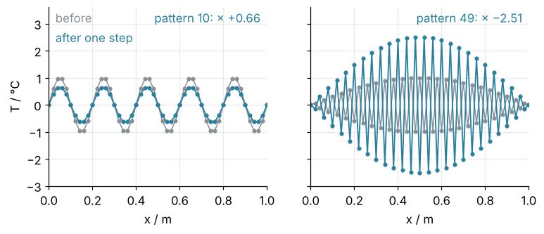
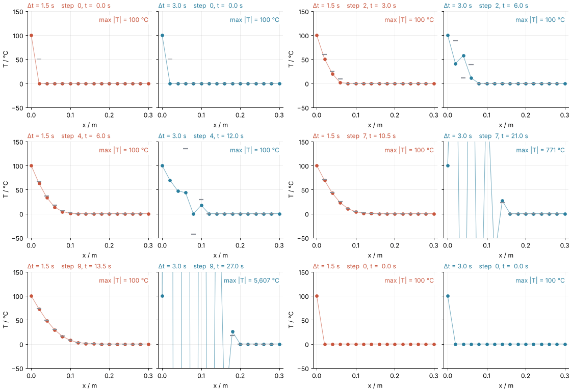
Pattern 10 comes out at 0.66 of its height, pattern 49 at −2.51 times its height, and both keep their shape. What is left to find is each pattern's factor, and which factors are larger than 1 in size. Here are the first ten steps of both runs near the hot end, each dot moving toward the mean of its neighbors:

"""Ten explicit steps near the hot end of the copper rod, at 1.5 s and at 3.0 s.

Renders ../../assets/rod-steps.gif for the finite differences Concept tutorial (py-finite-differences).
Each step: a gray tick appears at every dot's neighbors' mean, the dots slide to their new values,
the ticks fade. The rod is the one in index.md: 1 m of copper, 50 pieces, left end at 100 °C.
Run it from any directory:

    python scene.py
"""
from pathlib import Path

import numpy as np
import matplotlib.pyplot as plt
from matplotlib.animation import FuncAnimation, PillowWriter

OUT = Path(__file__).resolve().parents[2] / "assets" / "rod-steps.gif"
INK, ACCENT, SECOND, MUTED = "#1f2a44", "#c8553d", "#2a7f9e", "#8a8f98"
plt.rcParams.update({"axes.spines.top": False, "axes.spines.right": False,
                     "axes.grid": True, "grid.alpha": 0.25, "font.size": 11})

# ---- the rod of the tutorial
L, D, n, T_hot = 1.0, 1.17e-4, 50, 100.0
dx = L / n
x = np.linspace(0, L, n + 1)
shown = 16                                   # grid points in view: x from 0 to 0.3 m
n_steps = 10


def history(dt):
    """Profiles after 0 to n_steps explicit steps, ends included, and the neighbors' means before each step."""
    r = D * dt / dx**2
    T = np.zeros(n + 1)
    T[0] = T_hot
    profiles, means = [T.copy()], []
    for _ in range(n_steps):
        mean = 0.5 * (T[:-2] + T[2:])        # what each interior point moves toward
        means.append(mean)
        T[1:-1] = T[1:-1] + 2 * r * (mean - T[1:-1])
        profiles.append(T.copy())
    return np.array(profiles), np.array(means)


runs = [(1.5, ACCENT), (3.0, SECOND)]
data = [history(dt) for dt, _ in runs]

# ---- frame schedule: per step 2 frames for the ticks to appear, 6 to slide, 1 with the ticks gone
schedule = []                                # (step, phase, fraction)
for step in range(n_steps):
    schedule += [(step, "ticks", f) for f in (0.5, 1.0)]
    schedule += [(step, "slide", f) for f in np.linspace(1 / 6, 1, 6)]
    schedule += [(step, "settle", 1.0)]
schedule += [(n_steps, "hold", 1.0)] * 4
schedule += [(n_steps, "fade", f) for f in np.linspace(0.2, 1, 5)]   # the run fades out
schedule += [(0, "return", f) for f in np.linspace(0.25, 1, 4)]     # the cold rod fades in

# ---- figure, drawn once
fig, axes = plt.subplots(1, 2, figsize=(7.0, 3.2), dpi=80, sharey=True, layout="constrained")   # 560 x 256 px
artists = []
for ax, (dt, color) in zip(axes, runs):
    ax.set(xlim=(-0.01, x[shown - 1] + 0.01), ylim=(-50, 150), xlabel="x / m")
    (line,) = ax.plot([], [], "-", color=color, lw=1, alpha=0.6)
    (dots,) = ax.plot([], [], "o", color=color, ms=5)
    ticks = ax.hlines(np.zeros(shown - 2), x[1:shown - 1] - 0.006, x[1:shown - 1] + 0.006,
                      color=MUTED, lw=2)
    title = ax.set_title("", loc="left", fontsize=11, color=color)
    readout = ax.text(0.97, 0.95, "", transform=ax.transAxes, ha="right", va="top", color=color, zorder=5,
                      bbox=dict(fc="white", ec="none", alpha=0.85, pad=2))   # stays legible over the zigzag
    artists.append((line, dots, ticks, title, readout))
axes[0].set_ylabel("T / °C")


def update(i):
    step, phase, f = schedule[i]
    for (dt, color), (profiles, means), (line, dots, ticks, title, readout) in zip(runs, data, artists):
        before = profiles[step]
        after = profiles[min(step + 1, n_steps)]
        if phase == "slide":
            T, shown_step = before + f * (after - before), step + f
        elif phase in ("settle", "hold", "fade"):
            T, shown_step = after if phase == "settle" else before, step + (phase == "settle")
        else:                                 # "ticks", "return": the profile before the step
            T, shown_step = before, step
        alpha = 1.0
        if phase == "fade":
            alpha = 1 - f
        elif phase == "return":
            alpha = f
        dots.set_data(x[:shown], T[:shown])
        line.set_data(x[:shown], T[:shown])
        dots.set_alpha(alpha)
        line.set_alpha(0.6 * alpha)
        if phase in ("ticks", "slide") and step < n_steps:
            mean = means[step][:shown - 2]
            segs = [[(xi - 0.006, mi), (xi + 0.006, mi)] for xi, mi in zip(x[1:shown - 1], mean)]
            ticks.set_segments(segs)
            ticks.set_alpha(f if phase == "ticks" else 1.0)
        else:
            ticks.set_alpha(0.0)
        k = int(round(shown_step))
        title.set_text(f"Δt = {dt} s    step {k:2d}, t = {k * dt:4.1f} s")
        readout.set_text(f"max |T| = {np.abs(T).max():,.0f} °C")
        readout.set_alpha(alpha)


OUT.parent.mkdir(exist_ok=True)
FuncAnimation(fig, update, frames=len(schedule)).save(OUT, writer=PillowWriter(fps=12))
plt.close(fig)
print(f"{len(schedule)} frames, {OUT.stat().st_size / 1e6:.2f} MB")

Formalization

The rule of the previous sections is a finite difference. Add the Taylor series of \(T(x_j + \Delta x)\) and \(T(x_j - \Delta x)\), and the odd terms cancel:

The error falls with \(\Delta x^2\), second order, and vanishes for a straight line, whose fourth derivative is zero. That is why the steady state comes out exact on any grid.

For the 49 interior points at once the rule is \(dT/dt = D\,(AT + b)\). Here \(A\) is tridiagonal, with −2 on the diagonal and 1 beside it, all over \(\Delta x^2\), and \(b\) carries the hot end, 100 °C/\(\Delta x^2\) in its first entry:

print("dx² · A, top-left corner:")
print((dx**2 * A[:5, :5]).astype(int))
print(f"b[:3] = {b[:3]} °C/m²")

dx² · A, top-left corner:
[[-2  1  0  0  0]
 [ 1 -2  1  0  0]
 [ 0  1 -2  1  0]
 [ 0  0  1 -2  1]
 [ 0  0  0  1 -2]]
b[:3] = [250000.      0.      0.] °C/m²

One explicit step, \(T \leftarrow T + \Delta t\,D\,(AT + b)\), is then a matrix-vector product. The steady state \(T_s\) solves \(AT_s = -b\). Subtract it, and the deviation \(e = T - T_s\) obeys the plain update \(e \leftarrow (I + \Delta t\,D\,A)\,e\), with \(b\) gone.

\(A\) is symmetric, and its eigenvectors are the patterns of the previous section, \(v_j = \sin(k\pi x_j/L)\) for \(k\) = 1 to 49. Insert one into the second difference, and the sum formula for \(\sin(a \pm b)\) turns \(v_{j-1} + v_{j+1}\) into \(2\cos(k\pi\Delta x/L)\,v_j\). Subtract \(2v_j\) and halve the angle with \(\Delta x/L = 1/n\):

with \(n\) = 50 pieces. The eigenvalues that NumPy computes agree:

lam = -4 / dx**2 * np.sin(k * np.pi / (2 * n))**2
lam_numpy = np.linalg.eigvalsh(A)                               # ascending: most negative first
print(f"lambda_1  = {lam[0]:10.2f} 1/m²   lambda_49 = {lam[-1]:10.0f} 1/m²")
print(f"largest difference from eigvalsh: {np.abs(np.sort(lam) - lam_numpy).max():.1e} 1/m²")

dt_max = 2 / (D * abs(lam[-1]))
print(f"dt_max = 2/(D|lambda_49|) = {dt_max:.3f} s,   dx²/(2D) = {dx**2 / (2 * D):.3f} s")
print(f"slowest pattern decays in 1/(D|lambda_1|) = {1 / (D * abs(lam[0])):.0f} s; "
      f"one hour needs at least {int(np.ceil(3600 / dt_max)):,} steps")
for dt in [1.5, 3.0]:
    g = 1 + dt * D * lam
    print(f"dt = {dt} s: g_49 = {g[-1]:+.2f}")
g_impl = 1 / (1 - 60 * D * lam)
print(f"implicit, dt = 60 s: g_1 = {g_impl[0]:.3f} (exact decay {np.exp(-60 * D * abs(lam[0])):.3f}), "
      f"g_49 = {g_impl[-1]:.3f}")
dx_fine = L / 100
print(f"100 pieces of 1 cm: dt_max = {2 / (D * 4 / dx_fine**2 * np.sin(99 * np.pi / 200)**2):.2f} s")

# the 3.0 s run, pattern by pattern: share times g_k to the tenth power
g3 = 1 + 3.0 * D * lam
growing = k[np.abs(g3) > 1]
after10 = share * g3**10
print(f"\nat 3.0 s, |g| > 1 for patterns {growing[0]} to {growing[-1]} "
      f"(g from {g3[growing[0] - 1]:.2f} to {g3[-1]:.2f})")
print(f"step 10, pattern 49 alone:          {abs(after10[-1]):7,.0f} °C")
print(f"step 10, largest single pattern:    {np.abs(after10).max():7,.0f} °C (pattern {k[np.argmax(np.abs(after10))]})")
print(f"step 10, patterns 28 to 49 summed:  {np.abs(after10[27:] @ modes[27:]).max():7,.0f} °C")
print(f"step 10, the run itself:            {np.abs(unstable[10]).max():7,.0f} °C")

lambda_1  =      -9.87 1/m²   lambda_49 =      -9990 1/m²
largest difference from eigvalsh: 7.3e-12 1/m²
dt_max = 2/(D|lambda_49|) = 1.711 s,   dx²/(2D) = 1.709 s
slowest pattern decays in 1/(D|lambda_1|) = 866 s; one hour needs at least 2,104 steps
dt = 1.5 s: g_49 = -0.75
dt = 3.0 s: g_49 = -2.51
implicit, dt = 60 s: g_1 = 0.935 (exact decay 0.933), g_49 = 0.014
100 pieces of 1 cm: dt_max = 0.43 s

at 3.0 s, |g| > 1 for patterns 28 to 49 (g from -1.08 to -2.51)
step 10, pattern 49 alone:              615 °C
step 10, largest single pattern:      2,289 °C (pattern 44)
step 10, patterns 28 to 49 summed:   16,758 °C
step 10, the run itself:             16,708 °C

For an eigenvector, \(Av = \lambda_k v\), so one step maps \(v\) to \(v + \Delta t\,D\,\lambda_k v\). Any profile is a sum of the 49 patterns, and the step multiplies each by its own factor

independently of the others. Pattern 49 is the zigzag of the previous section under a slow sine envelope, and its factor −2.51 at 3.0 s is the \(1 - 4r\) found there, now with the exact \(\sin^2\). Stiffness draws the same factor as a stability region.

The limit comes from the fastest pattern, whatever the temperature and however long you run. \(|g_{49}| \le 1\) gives \(\Delta t \le 2/(D|\lambda_{49}|)\) = 1.711 s. The cruder bound \(r \le 1/2\), which replaces \(\sin^2\) by 1, gives \(\Delta x^2/(2D)\) = 1.709 s. Nothing in \(g_k\) depends on the amplitude, so a rod at 1,000 °C fails at the same step size as one at 1 °C. After \(N\) steps a pattern is \(g_k^N\) times its start: with \(|g_k| > 1\) it grows without bound from any seed, with \(|g_k| < 1\) it decays however long you run. The slowest pattern decays in 866 s and sets how long you must run, the fastest sets how short you must step: an hour at 1.711 s per step is at least 2,104 steps. At 3.0 s, every pattern from 28 to 49 has \(|g_k| > 1\), from 1.08 to 2.51. Pattern 49 alone reaches only 615 °C by step 10 and pattern 44 reaches 2,289 °C, while the band from 28 to 49 sums to 16,758 °C, within 0.3 % of the run's 16,708 °C. The threshold belongs to the fastest pattern; the size of the explosion belongs to the band.

Finer grids pay twice. \(\lambda_{49}\) scales as \(1/\Delta x^2\). With 100 pieces of 1 cm the limit drops to 0.43 s: twice the points and four times the steps, eight times the work for the same hour.

The implicit step removes the limit. Evaluate the right side at the new time instead of the old, \(T_\text{new} = T + \Delta t\,D\,(A T_\text{new} + b)\), and the unknown appears on both sides. Collected, it is the linear system

On an eigenvector the same one-line argument gives the factor \(1/(1 - \Delta t\,D\,\lambda_k)\), between 0 and 1 for every \(\Delta t\) because every \(\lambda_k\) is negative. With \(\Delta t\) = 60 s, 60 steps cover the hour, and pattern 49 is multiplied by 0.014 per step instead of amplified. The price is one tridiagonal solve per step. Accuracy, not stability, now limits the step: pattern 1 keeps 0.935 of itself per step where the heat equation keeps 0.933.

All 49 factors at once:

Show code

Copy

fig, ax = plt.subplots(figsize=(7, 3.6))
ax.axhspan(-1, 1, color=MUTED, alpha=0.15, lw=0)
for level in [-1, 1]:
    ax.axhline(level, color=MUTED, ls="--", lw=1)
for dt, color, label in [(1.5, ACCENT, "explicit, 1.5 s"), (3.0, SECOND, "explicit, 3.0 s")]:
    g = 1 + dt * D * lam
    ax.plot(k, g, "o", color=color, ms=4, label=label)
    ax.annotate(f"{g[-1]:+.2f}".replace("-", "−"), (k[-1], g[-1]), xytext=(6, 0), textcoords="offset points",
                va="center", color=color)
ax.plot(k, g_impl, "o", color=INK, ms=4, label="implicit, 60 s")
ax.set(xlabel="pattern k", ylabel="factor per step g", xlim=(0, 53), ylim=(-2.8, 1.4))
ax.legend(frameon=False, loc="lower left")
plt.show()

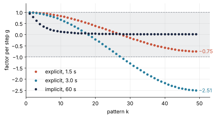
At 1.5 s every factor stays inside the band between −1 and 1, the lowest at −0.75. The implicit factors stay between 0 and 1, closer to 0 the finer the pattern.

See it in code

The matrix has 145 nonzero entries out of 2,401, so in practice it is stored sparse. scipy.sparse.diags_array builds it from its three diagonals, in CSC, the compressed column storage the sparse solver expects. scipy.sparse.linalg.factorized factors \(I - \Delta t\,D\,A\) once and returns a function that solves with it, called here once per step:

from scipy import sparse
from scipy.sparse.linalg import factorized

A_sp = sparse.diags_array([1.0, -2.0, 1.0], offsets=[-1, 0, 1], shape=(m, m), format="csc") / dx**2
print(f"A: {A_sp.shape[0]} x {A_sp.shape[1]}, {A_sp.nnz} nonzeros stored")
target = T_line[1:-1]

dt, n_steps = 1.5, 2400                                # explicit
T = np.zeros(m)
for _ in range(n_steps):
    T = T + dt * D * (A_sp @ T + b)
print(f"explicit, dt = {dt:4.1f} s, {n_steps:5,d} steps: max |T - line| = {np.abs(T - target).max():.2f} °C")

dt, n_steps = 60.0, 60                                 # implicit
solve = factorized(sparse.eye_array(m, format="csc") - dt * D * A_sp)
T = np.zeros(m)
for _ in range(n_steps):
    T = solve(T + dt * D * b)
print(f"implicit, dt = {dt:4.1f} s, {n_steps:5,d} steps: max |T - line| = {np.abs(T - target).max():.2f} °C")

slow = np.exp(-3600 * D * (np.pi / L)**2)               # pattern 1 of the heat equation itself
print(f"heat equation: pattern 1 starts at {abs(share[0]):.1f} °C, "
      f"after one hour x {slow:.4f} = {abs(share[0]) * slow:.2f} °C")

A: 49 x 49, 145 nonzeros stored
explicit, dt =  1.5 s, 2,400 steps: max |T - line| = 0.99 °C
implicit, dt = 60.0 s,    60 steps: max |T - line| = 1.14 °C
heat equation: pattern 1 starts at 63.6 °C, after one hour x 0.0157 = 1.00 °C

Both runs end near the straight line, the explicit one 0.99 °C from it after 2,400 steps, the implicit one 1.14 °C after 60, forty times fewer. The remaining deviation is not a discretization error. It is pattern 1, which started at 63.6 °C and after an hour of the true heat equation is still 1.00 °C high. The implicit run is 0.14 °C further off because its long step damps pattern 1 a little too slowly, which is the accuracy limit of the previous section. The same matrix in two dimensions, built with kron, is in Poisson's equation with scipy.sparse.

Where it shows up

The rod is one case of a diffusion equation, and every diffusion equation discretized on a grid inherits the same matrix and the same limit.

• Magnetic fields in conductors (physics). A magnetic field entering a copper plate obeys \(\partial B/\partial t = \eta\,\nabla^2 B\), with magnetic diffusivity \(\eta = 1/(\mu_0\sigma)\) ≈ 0.013 m²/s, over a hundred times the thermal one. Across the plate's thickness, a one-dimensional grid of 1 mm limits the explicit step to 37 µs, and a three-dimensional grid of 1 mm cells to 12 µs, so eddy-current codes step implicitly.
• Solutes in water and tissue (chemistry, biology). Fick's second law, \(\partial c/\partial t = D\,\nabla^2 c\), is the heat equation with concentration for temperature, and \(D\) ≈ 10⁻⁹ m²/s for small molecules in water. A three-dimensional grid of 10 µm cells allows explicit steps of 0.017 s, comfortable for one cell and expensive for hours of drug release from a gel.
• Groundwater (geology). The water level in a confined aquifer obeys a diffusion equation whose diffusivity is the aquifer's transmissivity divided by its storativity. MODFLOW, the U.S. Geological Survey's groundwater code, steps it implicitly, so that decades of pumping can be run in steps of days.
• Heat in electronics (engineering). Silicon conducts heat with a diffusivity near 9 × 10⁻⁵ m²/s, and a three-dimensional chip model with 10 µm cells has an explicit limit of about 0.19 µs, against power cycles that last seconds. Thermal solvers for packages step implicitly.
• Option pricing (mathematics). A change of variables turns the Black-Scholes equation into the heat equation, with the logarithm of the price as position and \(\sigma^2/2\) as diffusivity, \(\sigma\) being the volatility. The standard scheme there is Crank-Nicolson, the average of the explicit and the implicit step, published in 1947 for heat conduction.

Whatever the field calls its diffusivity \(D\), the explicit step on a grid in \(d\) dimensions is bounded by \(\Delta x^2/(2dD)\): a point has \(2d\) neighbors, so the zigzag's factor is \(1 - 4dr\), which must not fall below −1, and the implicit step trades the bound for one linear solve per step.

Further reading

• scipy.sparse.diags_array and scipy.sparse.linalg.factorized.
• LeVeque, Finite Difference Methods for Ordinary and Partial Differential Equations (SIAM, 2007), for stability beyond one rod.
• Langtangen and Linge, Finite Difference Computing with PDEs (Springer, 2017, open access), diffusion chapter.
• py-pde from the ground up: the heat equation on a square plate, whose Step 3 time step is this limit with four neighbors.
• Stiffness: why an explicit solver crawls on a reaction that has long settled and Eigenvalues with numpy.linalg: normal modes of coupled oscillators.
• More PDEs on this site: Finite volumes: why a conservation law is solved by bookkeeping the fluxes; The wave equation with leapfrog finite differences: a pulse on a string; Poisson's equation with scipy.sparse: two plates in a grounded box; Surface temperature of an airless planet: day, night, and below the ground, the same kind of matrix stepped implicitly.
• Planned: Finite differences in Julia.
• Download the notebook. It was executed with the library versions in the header.