Gradient descent: walking downhill, and why a narrow valley slows it down

The question

To find the lowest point of a landscape you cannot see, feel the slope where you stand and take a step against it. That is gradient descent, the simplest minimizer there is and the one that trains neural networks. The rule fits in one line: the step points downhill, and its length is a fixed number η, the step size, times the steepness of the slope. Here it is on two landscapes of two variables, x and y, from the same start at (−1.2, 1). Both have their lowest point at (1, 1). The first is a round bowl, \(f = (x - 1)^2 + (y - 1)^2\). The second is Rosenbrock's valley, \(f = (1 - x)^2 + 100\,(y - x^2)^2\), a narrow banana-shaped trough whose floor follows the parabola \(y = x^2\). Rosenbrock published the function in 1960, and it has been the standard trap for minimizers ever since, usually from that very start.

Each landscape gets the same treatment for the step size: three quarters of the largest step it tolerates at its minimum. That is η = 0.75 on the bowl and η = 0.0015 on the valley. Up to that limit a larger step arrives somewhat sooner. Past it the walker never settles at the minimum, as you will see.

Show code

Copy

import numpy as np
import matplotlib.pyplot as plt

plt.rcParams.update({
    "figure.figsize": (7, 3.6), "figure.dpi": 110,
    "axes.spines.top": False, "axes.spines.right": False,
    "axes.grid": True, "grid.alpha": 0.25,
    "font.size": 11, "lines.linewidth": 1.8,
})
INK, ACCENT, SECOND, MUTED = "#1f2a44", "#c8553d", "#2a7f9e", "#8a8f98"

# Two landscapes with the same minimum, (1, 1), each with its gradient and Hessian by hand.
def bowl(p):
    x, y = p
    return (x - 1)**2 + (y - 1)**2

def bowl_grad(p):
    x, y = p
    return np.array([2 * (x - 1), 2 * (y - 1)])

def bowl_hess(p):
    return np.array([[2.0, 0.0], [0.0, 2.0]])

def valley(p):                                   # Rosenbrock's function
    x, y = p
    return (1 - x)**2 + 100 * (y - x**2)**2

def valley_grad(p):
    x, y = p
    return np.array([-2 * (1 - x) - 400 * x * (y - x**2), 200 * (y - x**2)])

def valley_hess(p):
    x, y = p
    return np.array([[2 - 400 * (y - x**2) + 800 * x**2, -400 * x], [-400 * x, 200.0]])

x_min = np.array([1.0, 1.0])
x0 = np.array([-1.2, 1.0])                       # the usual start on Rosenbrock's function

def descend(grad, x0, eta, tol=1e-4, max_steps=100_000):
    """Fixed-step gradient descent; stops within tol of the known minimum (a real solver tests the gradient)."""
    path = [np.array(x0, float)]
    while np.linalg.norm(path[-1] - x_min) >= tol and len(path) <= max_steps:
        path.append(path[-1] - eta * grad(path[-1]))
        if np.abs(path[-1]).max() > 1e6:         # it has left for good
            break
    return np.array(path)

eta_bowl, eta_valley = 0.75, 0.0015              # three quarters of each landscape's largest stable step
walk_bowl = descend(bowl_grad, x0, eta_bowl)
walk_valley = descend(valley_grad, x0, eta_valley)
print(f"round bowl:        eta = {eta_bowl:<7}  {len(walk_bowl) - 1:6,d} steps")
print(f"Rosenbrock valley: eta = {eta_valley:<7}  {len(walk_valley) - 1:6,d} steps")
offset = walk_valley[:10, 1] - walk_valley[:10, 0]**2
print("valley walk, height above the floor y - x² at steps 0 to 9:", " ".join(f"{v:+.3f}" for v in offset))
height = walk_valley[:, 1] - walk_valley[:, 0]**2
flips = np.nonzero(np.sign(height[1:]) != np.sign(height[:-1]))[0] + 1
print("steps at which it changes side:", ", ".join(str(k) for k in flips),
      f"(at x = {walk_valley[flips[-1], 0]:.3f})")
print(f"largest height above or below the floor after step 10: {np.abs(height[10:]).max():.4f}")

fig, axes = plt.subplots(1, 2, figsize=(8, 3.3), sharey=True, width_ratios=[3.9, 3.2], layout="constrained")
panels = [(axes[0], bowl, walk_bowl, eta_bowl, np.linspace(0.25, 7, 12), (-1.6, 2.3)),   # the first bowl step lands at x = 2.1
          (axes[1], valley, walk_valley, eta_valley, np.logspace(-1, 3, 13), (-1.6, 1.6))]
X, Y = np.meshgrid(np.linspace(-1.6, 2.3, 500), np.linspace(-0.5, 1.7, 300))
for ax, f, walk, eta, levels, xlim in panels:
    ax.contour(X, Y, f((X, Y)), levels=levels, colors=MUTED, linewidths=0.7)
    ax.plot(walk[:, 0], walk[:, 1], color=ACCENT, lw=1.2)
    ax.plot(walk[:20, 0], walk[:20, 1], "o", color=ACCENT, ms=4)
    ax.plot(*x0, "o", color=INK, ms=6)
    ax.plot(*x_min, "x", color=INK, ms=8, mew=2)
    ax.text(0.03, 0.96, f"η = {eta}, {len(walk) - 1:,} steps", transform=ax.transAxes, va="top",
            bbox=dict(fc="white", ec="none", alpha=0.85, pad=1.5))
    ax.set(xlabel="x", xlim=xlim, ylim=(-0.5, 1.7), aspect="equal")
axes[0].set_ylabel("y")
plt.show()

round bowl:        eta = 0.75         15 steps
Rosenbrock valley: eta = 0.0015   15,220 steps
valley walk, height above the floor y - x² at steps 0 to 9: -0.440 +0.364 -0.105 +0.077 -0.026 +0.027 -0.002 +0.013 +0.005 +0.009
steps at which it changes side: 1, 2, 3, 4, 5, 6, 7, 509 (at x = 0.009)
largest height above or below the floor after step 10: 0.0084

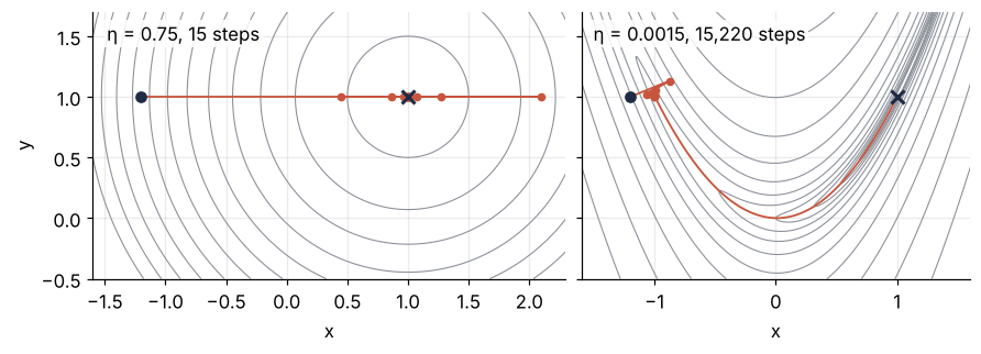
Both walkers arrive. On the bowl it takes 15 steps, each one jumping over the minimum and landing half as far away on the other side. In the valley the walker first hops back and forth across the valley a few times near the start, then follows the curved floor down through the origin and up the other arm to (1, 1). That takes 15,220 steps.

The rule is the same, and so is the minimum. So why does the valley tolerate only a step 500 times smaller than the bowl, why does that cost a thousand times more steps, and is there a better direction to step in than straight downhill?

The idea: step against the slope

The gradient \(\nabla f = (\partial f/\partial x,\ \partial f/\partial y)\) is the vector of the two partial derivatives. It points in the direction in which f rises fastest, and its length says how fast. Step against it and you go downhill as steeply as the ground allows. The walker knows nothing else: not where the minimum is, not what the ground looks like one step away, only the slope under its feet. Whether steepest downhill is also toward the minimum depends on the landscape. Here is the downhill direction, the arrow, against the straight line to the minimum at three points:

Show code

Copy

slopes = {}
points = [("round bowl", bowl, bowl_grad, x0, 1.0),
          ("valley wall", valley, valley_grad, np.array([0.6, 0.5]), 0.25),
          ("valley floor", valley, valley_grad, np.array([0.6, 0.36]), 0.25)]

fig, axes = plt.subplots(1, 3, figsize=(8, 3.0), layout="constrained")
for ax, (name, f, grad, p, half) in zip(axes, points):
    down = -grad(p)
    to_min = x_min - p
    angle = np.degrees(np.arccos(down @ to_min / np.linalg.norm(down) / np.linalg.norm(to_min)))
    slopes[name] = np.linalg.norm(down)
    print(f"{name:12s} at ({p[0]:+.2f}, {p[1]:.2f}):  |grad f| = {np.linalg.norm(down):6.2f},"
          f"  downhill is {angle:5.1f}° off the line to the minimum")
    x = np.linspace(p[0] - half, p[0] + half, 200)
    y = np.linspace(p[1] - half, p[1] + half, 200)
    Xl, Yl = np.meshgrid(x, y)
    ax.contour(Xl, Yl, f((Xl, Yl)), levels=12, colors=MUTED, linewidths=0.7)
    if f is valley:                                                   # the valley floor, y = x²
        ax.plot(x, x**2, ls="--", lw=1, color=MUTED)
    ax.plot([p[0], x_min[0]], [p[1], x_min[1]], ls="--", lw=1, color=INK)        # the line to the minimum
    d = 0.6 * half * down / np.linalg.norm(down)                     # normalized length
    ax.annotate("", p + d, p, arrowprops=dict(arrowstyle="-|>", color=INK, lw=1.8))
    ax.plot(*p, "o", color=INK, ms=5)
    ax.text(0.03, 0.97, f"{name}\n|∇f| = {np.linalg.norm(down):.2f}\nangle {angle:.1f}°",
            transform=ax.transAxes, va="top", bbox=dict(fc="white", ec="none", alpha=0.85, pad=1.5))
    ax.set(xlim=(x[0], x[-1]), ylim=(y[0], y[-1]), aspect="equal", xlabel="x")
axes[0].set_ylabel("y")
print(f"the slope on the wall is {slopes['valley wall'] / slopes['valley floor']:.0f} times the slope on the floor")
plt.show()

round bowl   at (-1.20, 1.00):  |grad f| =   4.40,  downhill is   0.0° off the line to the minimum
valley wall  at (+0.60, 0.50):  |grad f| =  44.35,  downhill is  90.5° off the line to the minimum
valley floor at (+0.60, 0.36):  |grad f| =   0.80,  downhill is  58.0° off the line to the minimum
the slope on the wall is 55 times the slope on the floor

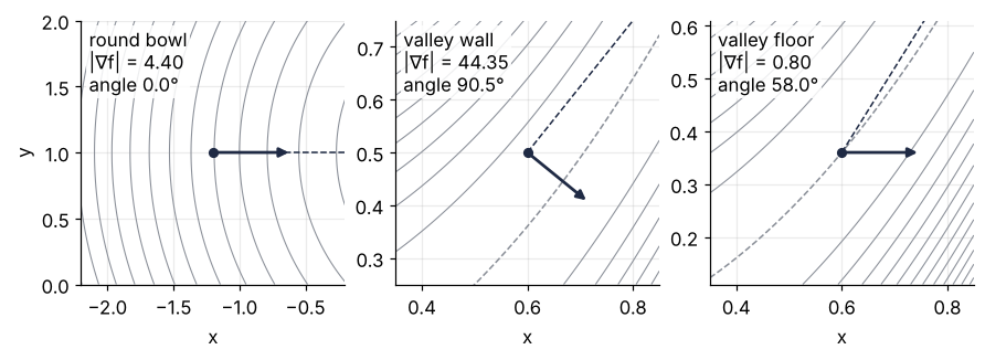
On the bowl the two coincide: the angle is 0°, and every step heads straight for the bottom. On the valley wall at (0.6, 0.5) the arrow is 90.5° off the line to the minimum. It points across the valley, toward the floor and the opposite wall, while the minimum lies up the valley. On the floor itself, 0.14 lower at (0.6, 0.36), the arrow points roughly up the valley, but the slope is 0.80 against 44.35 on the wall, 55 times gentler. The steep direction is the useless one.

The contour lines say why. Around the minimum of a smooth valley they are ellipses, long and thin here, and their two axes are the valley's principal directions. The short axis runs across the valley, where the ground curves up steeply on both sides. The long axis runs along the floor, where it barely curves at all. A geologist knows the idea from the principal axes of a strain ellipse. From here on these two are "across" and "along", with a curvature across and a curvature along. The valley bends, so the directions turn as you walk, but the picture holds at every point of the floor.

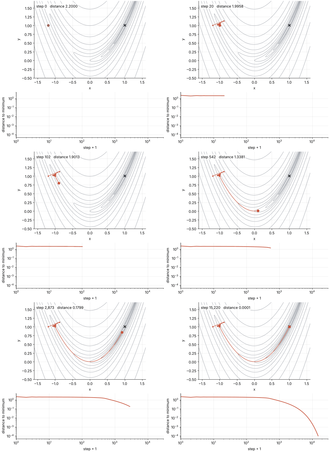
Watch the walker in the valley, one step per frame at first and then faster and faster:

"""Gradient descent in Rosenbrock's valley: a few bounces across the valley, then a long crawl along the floor.

Renders ../../assets/walker-valley.gif. Run it from any directory:

    python scene.py
"""
from pathlib import Path

import numpy as np
import matplotlib.pyplot as plt
from matplotlib.animation import FuncAnimation, PillowWriter
from PIL import Image

OUT = Path(__file__).resolve().parents[2] / "assets" / "walker-valley.gif"
INK, ACCENT, MUTED = "#1f2a44", "#c8553d", "#8a8f98"
plt.rcParams.update({"axes.spines.top": False, "axes.spines.right": False,
                     "axes.grid": True, "grid.alpha": 0.25, "font.size": 11})

# ---- the walk: fixed-step gradient descent from Rosenbrock's start, as in the tutorial
def valley(x, y):
    return (1 - x)**2 + 100 * (y - x**2)**2

def valley_grad(p):
    x, y = p
    return np.array([-2 * (1 - x) - 400 * x * (y - x**2), 200 * (y - x**2)])

x_min, eta = np.array([1.0, 1.0]), 0.0015
path = [np.array([-1.2, 1.0])]
while np.linalg.norm(path[-1] - x_min) >= 1e-4:
    path.append(path[-1] - eta * valley_grad(path[-1]))
path = np.array(path)
dist = np.linalg.norm(path - x_min, axis=1)
n = len(path) - 1

# ---- frames: every step up to 20, where the bounces are, then geometrically spaced to the end, the last held
steps = np.unique(np.concatenate([np.arange(21), np.geomspace(21, n, 80).round().astype(int)]))
frames = np.concatenate([steps, np.full(12, n)])

# ---- figure, drawn once
fig, (ax1, ax2) = plt.subplots(2, 1, figsize=(7, 6.4), dpi=80, height_ratios=[1.7, 1], layout="constrained")
X, Y = np.meshgrid(np.linspace(-1.6, 1.6, 400), np.linspace(-0.5, 1.7, 300))
ax1.contour(X, Y, valley(X, Y), levels=np.logspace(-1, 3, 13), colors=MUTED, linewidths=0.7)
ax1.plot(*x_min, "x", color=INK, ms=8, mew=2)
(trail,) = ax1.plot([], [], color=ACCENT, lw=1.2)
(hops,) = ax1.plot([], [], "o", color=ACCENT, ms=3)            # the first 20 steps as dots, to show the bounce
(walker,) = ax1.plot([], [], "o", color=ACCENT, ms=7)
counter = ax1.text(0.02, 0.96, "", transform=ax1.transAxes, va="top",
                   bbox=dict(fc="white", ec="none", alpha=0.85, pad=1.5))
ax1.set(xlabel="x", ylabel="y", xlim=(-1.6, 1.6), ylim=(-0.5, 1.7), aspect="equal")
(curve,) = ax2.plot([], [], color=ACCENT, lw=1.8)
ax2.set(xscale="log", yscale="log", xlim=(1, 2 * n), ylim=(5e-5, 5),
        xlabel="step + 1", ylabel="distance to minimum")

# ---- one frame: everything up to step k
def update(k):
    trail.set_data(path[:k + 1, 0], path[:k + 1, 1])
    hops.set_data(path[:min(k, 20) + 1, 0], path[:min(k, 20) + 1, 1])
    walker.set_data([path[k, 0]], [path[k, 1]])
    counter.set_text(f"step {k:,}   distance {dist[k]:.4f}")
    curve.set_data(np.arange(1, k + 2), dist[:k + 1])

# ---- render, and read back what was written
OUT.parent.mkdir(exist_ok=True)
FuncAnimation(fig, update, frames=frames).save(OUT, writer=PillowWriter(fps=12))
plt.close(fig)
with Image.open(OUT) as im:
    delay = im.info["duration"]
    print(f"{OUT.name}: {im.width} x {im.height} px, {im.n_frames} frames at {delay} ms, "
          f"{im.n_frames * delay / 1000:.1f} s, {OUT.stat().st_size / 1024:,.0f} kB")

The bounce is over almost at once. The walker's height above the floor, \(y - x^2\), flips sign at every step, from −0.440 at the start to +0.364, −0.105, +0.077, −0.026, and so on, until step 7. After that it changes side only once more, at step 509, without a jump, as it passes the bottom of the parabola at x = 0.009, and from step 10 on it is never farther than 0.0084 from the floor. The other 15,210 steps are the crawl along the floor. In the animation's lower panel the distance falls slowly while the walker goes down the left arm, then ever more steeply. That is not a speed-up. Near the end the walker loses the same fraction of its distance at every step, and each decade of the logarithmic step axis holds ten times as many steps as the one before, so the curve drops ever faster.

Too big a step, too small a step

The step size is the walker's one knob, and the valley restricts it from both sides. Here are four walks from the same start, each capped at the 15,220 steps the working walk needed:

Show code

Copy

n_cap = len(walk_valley) - 1                     # as many steps as the working walk needed
etas = [0.01, 0.003, 0.0015, 0.00015]
walks = {eta: descend(valley_grad, x0, eta, max_steps=n_cap) for eta in etas}

w = walks[0.01]
print(f"eta = 0.01:    after {len(w) - 1} steps |x| = {abs(w[-1, 0]):.2g}")
w = walks[0.003]
a, b = w[-1], w[-2]
period2 = np.linalg.norm(w[2:] - w[:-2], axis=1)
settled = np.nonzero(period2 > 1e-6)[0].max() + 1
print(f"eta = 0.003:   farthest along the floor x = {w[:, 0].max():.2f} at step {w[:, 0].argmax()}")
print(f"               from step {settled:,} on it alternates, to 1e-6, between")
for q in (a, b):
    print(f"               ({q[0]:.3f}, {q[1]:.3f}), height above the floor {q[1] - q[0]**2:+.3f}")
x_mid = (a[0] + b[0]) / 2
lam_across = np.linalg.eigvalsh(valley_hess(np.array([x_mid, x_mid**2])))[-1]
print(f"               distance to the minimum {np.linalg.norm(a - x_min):.2f}")
print(f"               floor point between them x = {x_mid:.3f}: curvature across = {lam_across:.1f},"
      f" 2/eta = {2 / 0.003:.1f}, factor 1 - eta*lambda = {1 - 0.003 * lam_across:+.2f}")
w = walks[0.00015]
print(f"eta = 0.00015: after {len(w) - 1:,} steps distance to the minimum {np.linalg.norm(w[-1] - x_min):.2f}")
w = descend(valley_grad, x0, 0.0019)             # just under the limit, not drawn
print(f"eta = 0.0019:  arrives after {len(w) - 1:,} steps")

style = {0.01: ":", 0.003: "-", 0.0015: "-", 0.00015: "--"}
far = walks[0.003][:, 0].argmax()                # the step after which η = 0.003 is thrown back
fig, (ax1, ax2) = plt.subplots(1, 2, figsize=(8, 3.5), width_ratios=[1.2, 1], layout="constrained")
ax1.contour(X, Y, valley((X, Y)), levels=np.logspace(-1, 3, 13), colors=MUTED, linewidths=0.7)
for eta, w in walks.items():
    color = ACCENT if eta == 0.0015 else INK
    if eta == 0.003:                             # the way down in full, the rattle after the throw-back faint
        ax1.plot(w[:far + 1, 0], w[:far + 1, 1], color=INK, lw=1.0)
        ax1.plot(w[far:, 0], w[far:, 1], color=INK, lw=0.6, alpha=0.3)
    else:
        shown = w[:3] if eta == 0.01 else w
        ax1.plot(shown[:, 0], shown[:, 1], ls=style[eta], color=color, lw=1.2, zorder=3 if eta == 0.0015 else 2)
    d = np.linalg.norm(w - x_min, axis=1)
    ax2.plot(np.arange(1, len(d) + 1), d, ls=style[eta], color=color)
    if eta == 0.00015:                           # both end at 0.48: this label goes where the two still differ
        ax2.text(2500, 6, f"η = {eta}", ha="center", color=color)
    else:
        ax2.text(len(d) * 1.3, d[-1], f"η = {eta}", va="center", color=color)
ax1.plot(*np.array([a, b]).T, "o-", color=INK, ms=5, lw=1.6, zorder=4)   # the two points of the η = 0.003 cycle
ax1.plot(*x0, "o", color=INK, ms=6)
ax1.plot(*x_min, "x", color=INK, ms=8, mew=2)
ax1.set(xlabel="x", ylabel="y", xlim=(-1.6, 1.6), ylim=(-0.5, 1.7), aspect="equal")
ax2.set(xscale="log", yscale="log", xlabel="step + 1", ylabel="distance to minimum",
        xlim=(1, 2e5), ylim=(1e-5, 1e10))
plt.show()

eta = 0.01:    after 4 steps |x| = 2.5e+08
eta = 0.003:   farthest along the floor x = 0.92 at step 829
               from step 3,747 on it alternates, to 1e-6, between
               (0.739, 0.597), height above the floor +0.051
               (0.786, 0.567), height above the floor -0.051
               distance to the minimum 0.48
               floor point between them x = 0.763: curvature across = 666.7, 2/eta = 666.7, factor 1 - eta*lambda = -1.00
eta = 0.00015: after 15,220 steps distance to the minimum 0.48
eta = 0.0019:  arrives after 11,994 steps

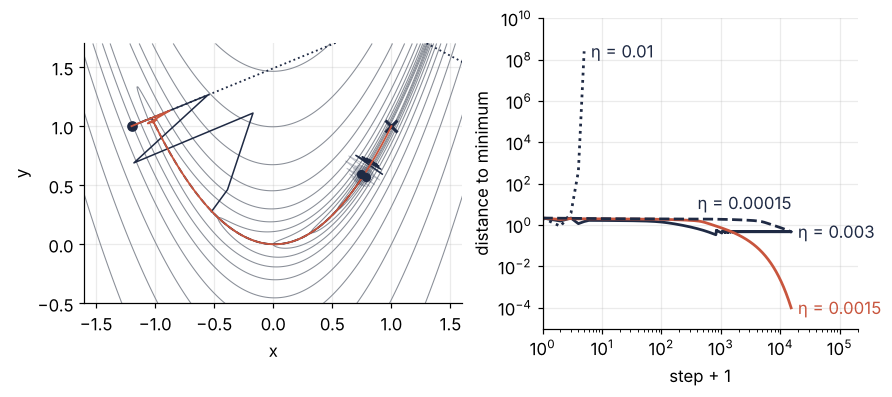
At η = 0.01 the first step throws the walker up the far wall, each next step farther, and after four steps it is at x = 2.5 × 10⁸. At η = 0.00015, one tenth of the working step, nothing goes wrong except time: after 15,220 steps the walker is still 0.48 from the minimum. A step just under the limit, η = 0.0019, does help, but not much: it arrives after 11,994 steps instead of 15,220.

The case in between is the instructive one. At η = 0.003 the walker gets down the valley and as far as x = 0.92 along the floor, at step 829, and is then thrown back. From step 3,747 on it jumps between the same two points, (0.739, 0.597) and (0.786, 0.567), 0.051 above the floor and 0.051 below it, and stays 0.48 from the minimum for good. That this is the same distance as the crawling walker's is a coincidence of this start.

The valley gets narrower, and its walls steeper, as it approaches the minimum. Farther out, a step of 0.003 across the floor lands on the other side closer to the floor than it started, and the bounce dies. Closer in, it lands farther away, and the bounce grows. Because the floor curves, the bounce also moves the walker along it: a step from above the floor goes forward and down, a step from below goes back and up. The point below lies nearer the minimum, where the walls are steeper, so the step back is the longer one. Once the bounce is large enough, that difference beats the gentle pull of the floor, and the walker is thrown back down the valley. At x = 0.763 a step across lands exactly as far from the floor as it started: the bounce stops growing, its backward push cancels the pull of the floor, and the walker stays for good.

The steep walls set the largest step that works, and that step is far too small for the gentle floor.

Formalization

As a formula, the walk is

with \(\mathbf x_k = (x_k, y_k)\) the position after k steps and η the step size. To see what one step does, you need a model of the landscape near a point. In one variable that is the Taylor expansion to second order,

a parabola with slope \(f'\) and curvature \(f''\). In two variables the slope becomes the gradient, and the curvature becomes a 2 × 2 table of second derivatives, the Hessian \(H\):

The term \(\mathbf s^{\mathsf T} H \mathbf s\) is the \(f'' s^2\) of one variable: the curvature in the direction of \(\mathbf s\), times its length squared. The principal directions of the valley, across and along, are what the literature calls the eigenvectors of \(H\), and the curvatures in them are its eigenvalues, \(\lambda_{\max}\) across and \(\lambda_{\min}\) along. The argument below needs one fact about them: near the minimum, a step that starts on a principal direction stays on it, so the walk splits into two one-variable walks.

lam_min, lam_max = np.linalg.eigvalsh(valley_hess(x_min))
kappa = lam_max / lam_min
print(f"valley Hessian at (1, 1): curvature across = {lam_max:.1f}, along = {lam_min:.3f}, kappa = {kappa:.0f}")
print(f"step limit 2/lambda_max: valley {2 / lam_max:.4f}, bowl {2 / 2:.1f};"
      f"  three quarters of it: {0.75 * 2 / lam_max:.4f}, {0.75 * 2 / 2:.2f}")
print(f"factor per step along the floor 1 - eta*lambda_min = {1 - eta_valley * lam_min:.6f};"
      f"  on the bowl 1 - eta*2 = {1 - eta_bowl * 2:+.2f}")
print(f"predicted steps per factor of 10: ln 10 / (eta * lambda_min) = {np.log(10) / (eta_valley * lam_min):,.0f}")
long_walk = descend(valley_grad, x0, eta_valley, tol=1e-6)
dist = np.linalg.norm(long_walk - x_min, axis=1)
first = [np.argmax(dist < tol) for tol in [1e-2, 1e-3, 1e-4, 1e-5, 1e-6]]
print("first step within 1e-2 ... 1e-6:", "  ".join(f"{n:,}" for n in first))
print("counted steps per factor of 10:  ", "  ".join(f"{n:,}" for n in np.diff(first)))

valley Hessian at (1, 1): curvature across = 1001.6, along = 0.399, kappa = 2508
step limit 2/lambda_max: valley 0.0020, bowl 1.0;  three quarters of it: 0.0015, 0.75
factor per step along the floor 1 - eta*lambda_min = 0.999401;  on the bowl 1 - eta*2 = -0.50
predicted steps per factor of 10: ln 10 / (eta * lambda_min) = 3,844
first step within 1e-2 ... 1e-6: 7,544  11,379  15,220  19,063  22,906
counted steps per factor of 10:   3,835  3,841  3,843  3,843

The step limit. Along a principal direction with curvature λ, the slope at distance d from the minimum is λd, so one step turns d into d − ηλd:

The walk converges only if the factor lies between −1 and 1 in both directions, which means \(\eta < 2/\lambda_{\max}\). In the valley at the minimum \(\lambda_{\max}\) = 1001.6 and the limit is 0.0020; on the bowl both curvatures are 2 and the limit is 1.0. When ηλ exceeds 1 the factor is negative: the walker overshoots, the bounce of the first steps. At ηλ = 2 exactly the factor is −1, and the bounce neither grows nor shrinks. The same holds locally: at x = 0.763, where the η = 0.003 walker stayed, the curvature across the floor is 666.7, which is 2/η itself, and the factor is −1.00.

The condition number counts the steps. Along the floor the curvature is \(\lambda_{\min}\) = 0.399 and the factor is \(1 - \eta\lambda_{\min}\) = 0.999401, so each factor of 10 in distance costs \(\ln 10 / (\eta\lambda_{\min})\) steps. Put in \(\eta = c \cdot 2/\lambda_{\max}\) with a fixed fraction c, and the count becomes \(\ln 10 \cdot \kappa / (2c)\), with \(\kappa = \lambda_{\max}/\lambda_{\min}\) the condition number of the Hessian. The valley has κ = 2508. The formula predicts 3,844 steps per factor of 10, and the walker, followed down to 10⁻⁶, counts 3,835, 3,841, 3,843 and 3,843. The bowl has κ = 1, and its factor is 1 − 0.75 · 2 = −0.50 in every direction: 15 steps in all. A narrow valley is a large κ, and κ is the bill.

The Newton step. Gradient descent uses the slope and ignores the curvature. Newton's method uses both. As in root finding, it looks for a zero, here of the slope: the point where ∇f = 0. In one variable the step divides the slope by the curvature,

and in two it does the same, direction by direction, which is what the inverse of the Hessian writes in one symbol:

Each step jumps to the bottom of the local quadratic model. On the bowl, which is its own quadratic model, that bottom is the minimum, reached in one step. On the valley it takes five:

Show code

Copy

def newton(grad, hess, x0, tol=1e-4):
    path = [np.array(x0, float)]
    while np.linalg.norm(path[-1] - x_min) >= tol:
        path.append(path[-1] - np.linalg.solve(hess(path[-1]), grad(path[-1])))
    return np.array(path)

newton_bowl = newton(bowl_grad, bowl_hess, x0)
newton_valley = newton(valley_grad, valley_hess, x0)
print(f"Newton on the round bowl: {len(newton_bowl) - 1} step")
print("Newton on the valley:")
for k, q in enumerate(newton_valley):
    line = f"  point {k}:  ({q[0]:+.3f}, {q[1]:+.3f})   f = {valley(q):9.4g}"
    if k < len(newton_valley) - 1:               # what the quadratic model at q promised for the next point
        g, H, s = valley_grad(q), valley_hess(q), newton_valley[k + 1] - q
        line += (f"   smallest curvature {np.linalg.eigvalsh(H)[0]:7.3f},"
                 f"  next step {np.linalg.norm(s):5.2f} long, model promises f = {valley(q) + g @ s + s @ H @ s / 2:9.4g}")
    print(line)

fig, ax = plt.subplots(figsize=(7, 3.6))
ax.contour(X, Y, valley((X, Y)), levels=np.logspace(-1, 3, 13), colors=MUTED, linewidths=0.7)
ax.plot(walk_valley[:, 0], walk_valley[:, 1], color=ACCENT, lw=1.2)
ax.text(-0.55, 0.5, "gradient descent", color=ACCENT)
ax.plot(newton_valley[:, 0], newton_valley[:, 1], "-", color=SECOND, lw=1.2)     # the axes clip the jump to step 2
on_map = newton_valley[:, 1] > -0.5
ax.plot(*newton_valley[on_map].T, "o", color=SECOND, ms=6)
ax.plot(*x0, "o", color=INK, ms=6)
for k in [0, 1, 3]:
    ax.annotate(str(k), newton_valley[k], xytext=(-12, 4), textcoords="offset points", color=SECOND)
ax.annotate("Newton", newton_valley[1], xytext=(8, 0), textcoords="offset points", va="center", color=SECOND)
ax.annotate("4, 5", newton_valley[4], xytext=(9, -14), textcoords="offset points", color=SECOND)  # 0.06 apart
q = newton_valley[2]
ax.annotate(f"2: ({q[0]:.2f}, {q[1]:.2f})\nf = {valley(q):.0f}".replace("-", "−"), (q[0], -0.5), xytext=(q[0] - 0.1, -0.2),
            ha="right", va="center", color=SECOND, arrowprops=dict(arrowstyle="-|>", color=SECOND, lw=1, relpos=(1, 0.5)))
ax.plot(*x_min, "x", color=INK, ms=8, mew=2)
ax.set(xlabel="x", ylabel="y", xlim=(-1.6, 1.6), ylim=(-0.5, 1.7), aspect="equal")
plt.show()

Newton on the round bowl: 1 step
Newton on the valley:
  point 0:  (-1.200, +1.000)   f =      24.2   smallest curvature  23.633,  next step  0.38 long, model promises f =     4.786
  point 1:  (-1.175, +1.381)   f =     4.732   smallest curvature   0.343,  next step  4.95 long, model promises f =    0.5153
  point 2:  (+0.763, -3.175)   f =      1412   smallest curvature 148.860,  next step  3.76 long, model promises f =   0.05604
  point 3:  (+0.763, +0.583)   f =   0.05597   smallest curvature   0.599,  next step  0.43 long, model promises f = 1.109e-06
  point 4:  (+1.000, +0.944)   f =    0.3132   smallest curvature   4.783,  next step  0.06 long, model promises f = 2.018e-11
  point 5:  (+1.000, +1.000)   f = 1.853e-11

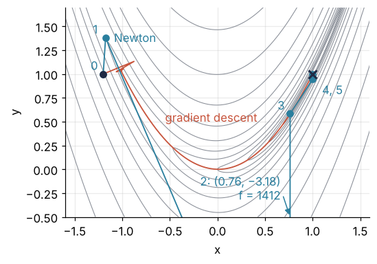
The second Newton step lands at point 2, far below the map at (0.763, −3.175), where f = 1412, uphill from 4.732 at point 1, and the fourth step climbs again, from 0.05597 to 0.3132. The landscape curves upward in every direction at all of these points, so each step aims at the bottom of a bowl, but the model's bowl. At point 1 the curvature along the floor is 0.343, dividing the slope by it gives a step 4.95 long, and out there the model promises f = 0.5153 where the valley has 1412. Where the landscape does not curve upward in every direction (the literature says \(H\) is not positive definite), it is worse: the model has no bottom at all, and the step heads for a maximum or a saddle. Practical methods therefore damp the Newton step, or build up the curvature from earlier gradients. BFGS, the default of scipy.optimize.minimize, does the second.

See it in code

SciPy has no plain gradient descent; scipy.optimize.minimize offers better methods instead. The check is therefore twenty lines of NumPy that run both walkers on the bowl and on SciPy's own Rosenbrock function, whose exact gradient and Hessian come as rosen_der and rosen_hess, followed by BFGS through minimize:

import numpy as np
from scipy.optimize import rosen, rosen_der, rosen_hess, minimize

def gradient_descent(grad, x, eta, tol=1e-4):
    steps = 0
    while np.linalg.norm(x - 1) >= tol:          # both minima are at (1, 1)
        x, steps = x - eta * grad(x), steps + 1
    return x, steps

def newton(grad, hess, x, tol=1e-4):
    steps = 0
    while np.linalg.norm(x - 1) >= tol:
        x, steps = x - np.linalg.solve(hess(x), grad(x)), steps + 1
    return x, steps

landscapes = [(lambda x: 2 * (x - 1), lambda x: 2 * np.eye(2), 0.75),   # round bowl: gradient, Hessian, eta
              (rosen_der, rosen_hess, 0.0015)]                          # SciPy's Rosenbrock derivatives
x0 = np.array([-1.2, 1.0])
print(f"{'':18s}{'round bowl':>36s}{'Rosenbrock valley':>36s}")
for name in ["gradient descent", "Newton"]:
    row = []
    for grad, hess, eta in landscapes:
        x, n = gradient_descent(grad, x0, eta) if name == "gradient descent" else newton(grad, hess, x0)
        row.append(f"{n:6,d} {'step ' if n == 1 else 'steps'}  ({x[0]:.5f}, {x[1]:.5f})")
    print(f"{name:18s}{row[0]:>36s}{row[1]:>36s}")
res = minimize(rosen, x0, jac=rosen_der)          # BFGS, the default without bounds
print(f"BFGS (minimize): {res.nit} iterations, x = ({res.x[0]:.5f}, {res.x[1]:.5f})")

                                            round bowl                   Rosenbrock valley
gradient descent          15 steps  (1.00007, 1.00000)    15,220 steps  (0.99996, 0.99991)
Newton                     1 step   (1.00000, 1.00000)         5 steps  (1.00000, 0.99999)
BFGS (minimize): 32 iterations, x = (1.00000, 1.00000)

All four walks end within 10⁻⁴ of (1, 1), and the counts are the ones from the start: 15 and 15,220 for gradient descent, one and five for Newton. SciPy's derivatives give the same counts as the hand-written ones, so those were right. BFGS needs 32 iterations with gradients alone, between Newton's five with the exact Hessian and gradient descent's 15,220. For real work on a smooth function, call minimize, as in Minimization with scipy.optimize.minimize, and keep the hand-written walker for understanding.

On your own function you do not know the curvature at the minimum, so the rule for η above is not available. Start with a guess and halve the step whenever f goes up, or let a line search choose the step anew at every iteration, which is what minimize does for BFGS.

Where it shows up

The walker in the valley is the picture behind most of the minimizing done in science: a misfit or an energy, many variables, and a slope you can compute.

• Fitting. A least-squares fit minimizes the sum of squared residuals over the parameters, as Least squares: what a fit minimizes, and why the residuals are squared explains. Gauss-Newton and Levenberg-Marquardt, the default of curve_fit without bounds and a method of scipy.optimize.least_squares, take Newton-like steps on it, and Levenberg-Marquardt shifts toward gradient descent when it stops trusting the Newton step.
• Neural networks. Training is gradient descent on a loss over millions of weights, with the learning rate as η and the gradient from backpropagation, the chain rule applied layer by layer from the output back to the input, estimated on small random batches of the data (stochastic gradient descent). The common refinements fight exactly the bounce across narrow valleys: momentum averages the recent steps, so that the back and forth across the valley cancels while the part along the floor adds up, and Adam also scales the step of each weight by the size of its recent gradients.
• Molecules and materials. Energy minimization before a molecular dynamics run is usually steepest descent (in GROMACS, integrator = steep), with conjugate gradients or L-BFGS when the structure must get closer to the minimum. The seven argon atoms of the minimize tutorial are the same problem at its smallest.
• Linear systems. Solving \(A\mathbf x = \mathbf b\) for a symmetric positive definite \(A\) is the same as minimizing \(\tfrac12 \mathbf x^{\mathsf T} A \mathbf x - \mathbf b^{\mathsf T} \mathbf x\), a quadratic valley whose Hessian is \(A\). Steepest descent on it needs a number of steps in proportion to κ, conjugate gradients in proportion to √κ, the subject of Conjugate gradients and the condition number.
• Inverse problems in geophysics and imaging. Full-waveform inversion and image reconstruction minimize a misfit over millions of unknowns with L-BFGS and other quasi-Newton methods. The gradient comes from an adjoint computation: one extra simulation, run backward in time, gives the derivative with respect to every unknown at once, instead of one run per unknown.

Every one of them steps against the slope, and the condition number of the Hessian decides how many steps it takes.

Further reading

• The SciPy reference for minimize and rosen, with rosen_der and rosen_hess next to it.
• Nocedal and Wright, Numerical Optimization, 2nd ed. (Springer, 2006), for gradient descent, Newton, line searches, and BFGS, with the convergence rates behind the condition number argument.
• Boyd and Vandenberghe, Convex Optimization (Cambridge, 2004), chapter 9, unconstrained minimization, free on the authors' web page.
• Related tutorials on this site: Minimization with scipy.optimize.minimize: the shape of a seven-atom cluster; Conjugate gradients and the condition number: why iterations grow as √κ; Least squares: what a fit minimizes, and why the residuals are squared; The condition number: how many digits a linear solve can lose; Root finding with scipy.optimize: Halley's comet from Kepler's equation, where Newton's method first appears.
• Download the notebook. It was executed with the library versions in the header.