The Barnes-Hut algorithm: how a tree cuts a galaxy's N² forces to N log N (Python)

The question

Here are 5,000 stars of a model disk galaxy, dense at the center and thinning out toward the edge. To move them one time step you need the gravitational pull on every star from every other star: 12,497,500 pairs. The Barnes-Hut algorithm gets the same forces, to 1.4 % for the median star, from 181 terms per star on average, and this tutorial is about how.

Show code

import datetime, json, os, platform, timeit
from collections import namedtuple

import numpy as np
import matplotlib.pyplot as plt
from matplotlib.collections import PatchCollection
from matplotlib.patches import Rectangle

plt.rcParams.update({
    "figure.figsize": (7, 3.6), "figure.dpi": 110,
    "axes.spines.top": False, "axes.spines.right": False,
    "axes.grid": True, "grid.alpha": 0.25,
    "font.size": 11, "lines.linewidth": 1.8,
})
INK, ACCENT, SECOND, MUTED = "#1f2a44", "#c8553d", "#2a7f9e", "#8a8f98"

# Units: G = 1, total mass 1, lengths in disk scale lengths R_d (think 3 kpc).
N, EPS = 5_000, 0.01                     # EPS: Plummer softening, so that two close stars stay finite

def disk(n, seed=20261009):
    """Positions and masses of n equal stars in an exponential disk, cut at 5 R_d."""
    rng = np.random.default_rng(seed)
    R = rng.gamma(2.0, 1.0, size=4 * n)  # surface density exp(-R) gives p(R) ~ R exp(-R)
    R = R[R < 5][:n]
    phi = rng.uniform(0, 2 * np.pi, n)
    return np.column_stack([R * np.cos(phi), R * np.sin(phi)]), np.full(n, 1 / n)

def direct(pos, m, rows=None, chunk=500):
    """Acceleration on each star in rows (default: all) from all stars, summed pair by pair."""
    targets = pos if rows is None else pos[rows]
    acc = np.empty_like(targets)
    x, y = pos[:, 0], pos[:, 1]
    for s in range(0, len(targets), chunk):
        dx = x - targets[s:s + chunk, :1]           # a star's pull on itself is zero: dx = dy = 0
        dy = y - targets[s:s + chunk, 1:]
        r2 = dx**2 + dy**2 + EPS**2
        w = m / (r2 * np.sqrt(r2))
        acc[s:s + chunk, 0] = (w * dx).sum(axis=1)
        acc[s:s + chunk, 1] = (w * dy).sum(axis=1)
    return acc

pos, m = disk(N)

fig, ax = plt.subplots(figsize=(5, 5))
ax.scatter(pos[:, 0], pos[:, 1], s=1, color=INK, alpha=0.5, lw=0)
ax.set(xlabel="x / R_d", ylabel="y / R_d", xlim=(-5, 5), ylim=(-5, 5), aspect="equal")
plt.show()

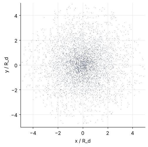
Map of 5,000 stars of a model disk galaxy, x and y from −5 to 5 disk scale lengths. The dots crowd into a dense core and thin out toward the rim.

The obvious way is the one from Vectorizing loops with NumPy: every star against every other, in chunks of 500 rows so the arrays fit in memory. Each squared distance gets a small ε² = (0.01 R_d)² added, the softening, so that two stars passing very close do not pull with an almost infinite force. The times below were measured once, on the machine named in the output, and are stored in timings.json, so that the page shows the same numbers on every rebuild.

Show code

TIMINGS = "timings.json"
if os.path.exists(TIMINGS):
    with open(TIMINGS) as f:
        timings = json.load(f)
else:
    timings = {"date": str(datetime.date.today()),
               "machine": f"{platform.machine()}, {os.cpu_count()} cores, "
                          f"Python {platform.python_version()}, NumPy {np.__version__}"}

def best_time(label, func, repeat=3):
    # returns the STORED time if label is in timings.json: delete the file after changing code
    if label not in timings:
        timings[label] = float(f"{min(timeit.repeat(func, number=1, repeat=repeat)):.2g}")
        with open(TIMINGS, "w") as f:
            json.dump(timings, f, indent=1)
    return timings[label]

a_direct = direct(pos, m)
half_pos, half_m = disk(N // 2)
t_half = best_time("direct 2500", lambda: direct(half_pos, half_m))
t_full = best_time("direct 5000", lambda: direct(pos, m))
print(f"measured {timings['date']} on {timings['machine']}")
print(f"pairs for {N:,} stars: {N * (N - 1) // 2:,}")
print(f"direct sum, 2,500 stars: {t_half:.2g} s")
print(f"direct sum, 5,000 stars: {t_full:.2g} s   ratio {t_full / t_half:.1f}")

measured 2026-10-09 on x86_64, 4 cores, Python 3.12.3, NumPy 2.4.3
pairs for 5,000 stars: 12,497,500
direct sum, 2,500 stars: 0.18 s
direct sum, 5,000 stars: 0.65 s   ratio 3.6

Twice the stars, four times the pairs, and the clock says 3.6. A simulation runs thousands of steps, and a galaxy model of a million stars has 5 × 10¹¹ pairs in every one of them.

There is no way around the counting as long as every pair is its own term. But a far clump of stars should pull on a star almost like one heavy star at the clump's center of mass. The question is how to find those clumps for every star without looking at every pair first, and what accuracy the lumping costs.

The idea: a distant clump pulls like one star

Take the 34 stars in a square of side 0.5 R_d around (−2, 0) and the star closest to (2.5, 0) on the other side of the disk. Add up the 34 pulls one by one, then replace the clump by one star of the same total mass at its center of mass, and compare. The measure of the damage, here and everywhere below, is the relative force error: the length of the difference between the approximate and the exact acceleration, divided by the length of the exact one, \(|\mathbf a_\mathrm{approx} - \mathbf a_\mathrm{exact}| / |\mathbf a_\mathrm{exact}|\). Then do the same from two stars closer to the clump, with s the side of the square and d the distance to its center of mass:

Show code

def nearest(x, y):
    return np.argmin(np.hypot(pos[:, 0] - x, pos[:, 1] - y))

clump = np.flatnonzero((np.abs(pos[:, 0] + 2) < 0.25) & (np.abs(pos[:, 1]) < 0.25))
M_clump = m[clump].sum()
r_c = m[clump] @ pos[clump] / M_clump               # center of mass of the clump

def pull(masses, sources, r):
    d = sources - r
    r2 = (d**2).sum(axis=-1) + EPS**2
    return (masses[:, None] * d / (r2 * np.sqrt(r2))[:, None]).sum(axis=0)

target = nearest(2.5, 0)
print(f"{len(clump)} stars in the clump")
print("   star at      s/d    error")
for i in [target, nearest(0, 0), nearest(-1, 0)]:
    exact = pull(m[clump], pos[clump], pos[i])
    lumped = pull(np.array([M_clump]), r_c[None, :], pos[i])
    s_over_d = 0.5 / np.linalg.norm(r_c - pos[i])
    err = np.linalg.norm(lumped - exact) / np.linalg.norm(exact)
    print(f"({pos[i, 0]:+.2f}, {pos[i, 1]:+.2f})   {s_over_d:.3f}   {err:.1e}")

34 stars in the clump
   star at      s/d    error
(+2.52, +0.06)   0.110   1.0e-03
(+0.00, -0.01)   0.248   5.2e-03
(-0.99, +0.05)   0.490   2.3e-02

From the far side of the disk, where the square looks small, one mass instead of 34 costs a tenth of a percent. At s/d = 0.25 the error is five times larger, at 0.49 more than twenty times. Doubling s/d multiplies the error by about four: the error goes roughly as (s/d)².

That settles how good a clump is. Which clumps to use is the second half. Cut a square around the whole disk into four equal squares, each of those into four again, and keep cutting every square that holds more than one star. Each square stores three numbers you need later: its side, its total mass, and its center of mass. The result is a tree of nested squares, a quadtree, with the whole disk at the root and single stars at the leaves.

Show code

Tree = namedtuple("Tree", "cx cy side mass comx comy star children depth")

def build(pos, m):
    """Quadtree as flat lists: node k has center, side, mass, center of mass, and either a star or children."""
    t = Tree(*([] for _ in Tree._fields))
    def node(idx, cx, cy, half, level):
        k = len(t.side)
        M = m[idx].sum()
        com = m[idx] @ pos[idx] / M
        star = idx[0] if len(idx) == 1 else -1
        for field, value in zip(t, (cx, cy, 2 * half, M, com[0], com[1], star, [], level)):
            field.append(value)
        if star < 0:
            east, north = pos[idx, 0] >= cx, pos[idx, 1] >= cy
            for e in (False, True):
                for n in (False, True):
                    sub = idx[(east == e) & (north == n)]
                    if len(sub):
                        h = half / 2
                        t.children[k].append(node(sub, cx + (h if e else -h), cy + (h if n else -h), h, level + 1))
        return k
    node(np.arange(len(pos)), 0.0, 0.0, 1.0001 * np.abs(pos).max(), 0)
    return t

def squares(t, cells, **style):
    return PatchCollection([Rectangle((t.cx[k] - t.side[k] / 2, t.cy[k] - t.side[k] / 2), t.side[k], t.side[k])
                            for k in cells], **style)

tree = build(pos, m)
depth, leaf = np.array(tree.depth), np.array(tree.star) >= 0
print(f"nodes {len(tree.side):,}, leaves {leaf.sum():,}")
print(f"maximum depth {depth.max()}, mean leaf depth {depth[leaf].mean():.1f}, log4 N = {np.log(N) / np.log(4):.1f}")

fig, ax = plt.subplots(figsize=(5, 5))
ax.add_collection(squares(tree, range(len(tree.side)), facecolor="none", edgecolor=MUTED, lw=0.3))
ax.scatter(pos[:, 0], pos[:, 1], s=1, color=INK, alpha=0.5, lw=0)
ax.add_patch(Rectangle((-2.25, -0.25), 0.5, 0.5, facecolor="none", edgecolor=ACCENT, lw=1.6))
ax.plot(*pos[target], "o", color=INK, ms=7, mec="white", mew=1.5)
ax.set(xlabel="x / R_d", ylabel="y / R_d", xlim=(-5, 5), ylim=(-5, 5), aspect="equal")
ax.grid(False)
plt.show()

nodes 8,582, leaves 5,000
maximum depth 13, mean leaf depth 7.7, log4 N = 6.1

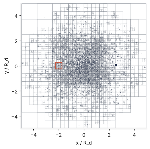
The quadtree over the disk, x and y from −5 to 5 R_d. Gray square outlines are large at the rim and shrink to tiny cells in the dense core. A red square marks the 34-star clump at x = −2, a dark dot the target star at x = 2.5.

8,582 squares for 5,000 stars. The cells stay large at the rim and shrink to slivers in the core, where the tree goes 13 levels deep.

The tree walk: accept a cell or open it

For one star, start at the root, the square around the whole disk, and ask whether it is small as seen from the star: is s/d below a chosen number θ? For a small cell s/d is the angle in radians the cell spans in the star's sky, so θ is literally an opening angle. If the cell passes, its whole content acts as one mass at its center of mass, and the walk is done with it. If not, open it and ask the same of each of its children. A leaf with one star is always summed directly, and the star skips itself. Each accepted cell or directly summed star is one interaction, one force evaluation; the direct sum needs 4,999 of them per star.

Show code

def walk(t, pos, i, theta, record=False):
    """Acceleration on star i and the number of interactions; with record, also the accepted nodes."""
    xi, yi = pos[i]
    ax = ay = 0.0
    accepted = []
    stack = [0]                                         # start at the root
    while stack:
        k = stack.pop()
        if t.star[k] == i:
            continue
        dx, dy = t.comx[k] - xi, t.comy[k] - yi
        d2 = dx * dx + dy * dy
        if t.star[k] >= 0 or t.side[k] ** 2 < theta**2 * d2:     # a single star, or s/d < theta
            f = t.mass[k] * (d2 + EPS**2) ** -1.5
            ax, ay = ax + f * dx, ay + f * dy
            accepted.append(k)
        else:
            stack.extend(t.children[k])                 # open the cell
    a = np.array([ax, ay])
    return (a, len(accepted), accepted) if record else (a, len(accepted))

Here is the walk for the star at x = 2.5 R_d at two settings. Shaded squares are cells taken as one mass, blue dots the stars summed one by one:

Show code

def rel_err(a, b):
    return np.linalg.norm(a - b, axis=-1) / np.linalg.norm(b, axis=-1)

def draw_walk(ax, theta, i=target, letter=""):
    a, n, cells = walk(tree, pos, i, theta, record=True)
    singles = [tree.star[k] for k in cells if tree.star[k] >= 0]
    lumps = [k for k in cells if tree.star[k] < 0]
    ax.scatter(pos[:, 0], pos[:, 1], s=1, color=INK, alpha=0.25, lw=0)
    ax.add_collection(squares(tree, lumps, facecolor=ACCENT, edgecolor=ACCENT, alpha=0.35, lw=0.6))
    ax.scatter(pos[singles, 0], pos[singles, 1], s=10, color=SECOND, lw=0)
    ax.plot(*pos[i], "o", color=INK, ms=7, mec="white", mew=1.5)
    ax.text(0, 1.03, f"{letter}θ = {theta}: {n} interactions, error {100 * rel_err(a, a_direct[i]):.2g} %",
            transform=ax.transAxes, va="bottom")
    ax.set(xlim=(-5, 5), ylim=(-5, 5), aspect="equal", xlabel="x / R_d")
    ax.grid(False)

fig, axes = plt.subplots(1, 2, figsize=(8, 4.2), sharey=True)
for ax, theta in zip(axes, [0.3, 0.8]):
    draw_walk(ax, theta)
axes[0].set_ylabel("y / R_d")
plt.show()

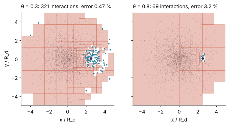
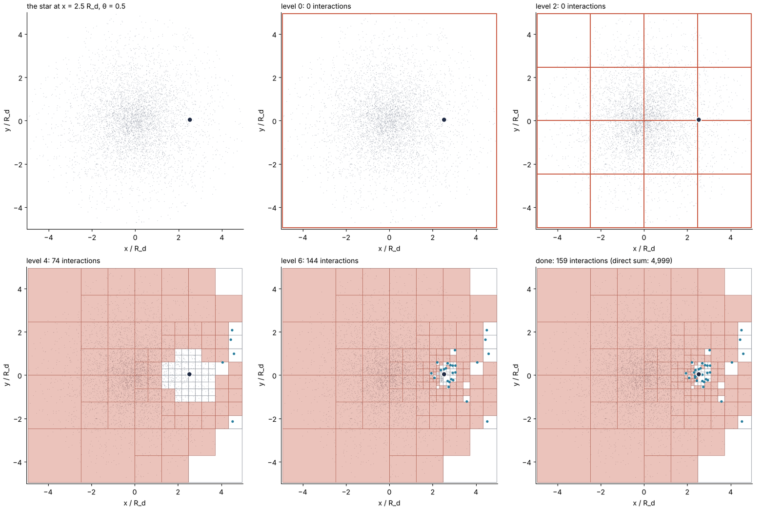
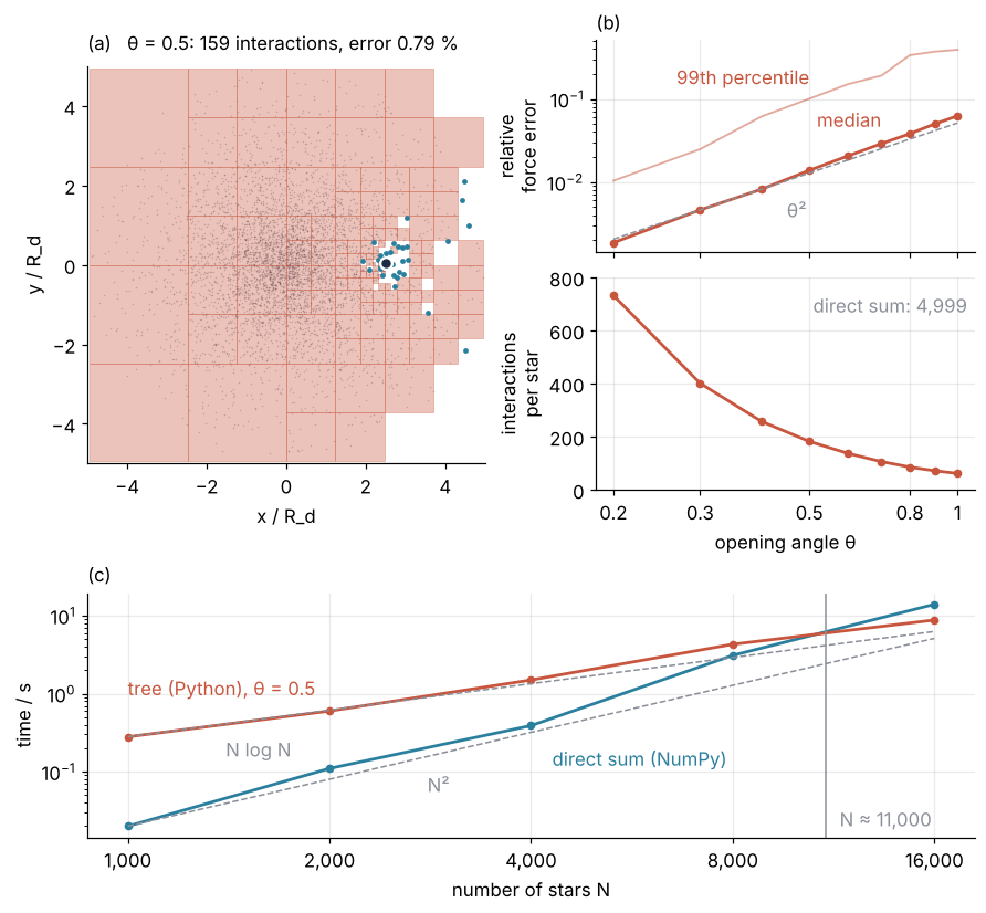
Two maps of the disk for the target star at x = 2.5 R_d. Left, θ = 0.3: many small red cells and dozens of blue single stars near the target, 321 interactions. Right, θ = 0.8: a few large red cells, 69 interactions, error 3.2 % against 0.47 %.

At θ = 0.3 the star needs 321 interactions and gets its force right to 0.47 %. At θ = 0.8 it needs 69, and the error grows to 3.2 %. Either way it is a small fraction of 4,999. The walk itself, level by level, at θ = 0.5:

The tree walk for the target star at θ = 0.5, one tree level after another. Cells under test light up in red outline; far cells are accepted and fill red in a few large squares, near cells split into four, and single stars close to the target turn blue. A counter adds up the interactions.

Show code

"""The Barnes-Hut tree walk for one star at theta = 0.5, one tree level at a time.

Renders ../../assets/tree-walk.gif for the Barnes-Hut Concept tutorial (py-barnes-hut).
The disk, the tree, and the opening criterion are the ones in index.md: 5,000 stars,
seed 20261009, one star per leaf, s/d < theta with d to the center of mass.
Run it from any directory:

    python scene.py
"""
from pathlib import Path

import numpy as np
import matplotlib.pyplot as plt
from matplotlib.animation import FuncAnimation, PillowWriter
from matplotlib.collections import PatchCollection
from matplotlib.patches import Rectangle

OUT = Path(__file__).resolve().parents[2] / "assets" / "tree-walk.gif"
INK, ACCENT, SECOND, MUTED = "#1f2a44", "#c8553d", "#2a7f9e", "#8a8f98"
plt.rcParams.update({"axes.spines.top": False, "axes.spines.right": False, "font.size": 11})
THETA = 0.5

# ---- the disk and the tree of the tutorial
rng = np.random.default_rng(20261009)
R = rng.gamma(2.0, 1.0, size=20_000)
R = R[R < 5][:5_000]
phi = rng.uniform(0, 2 * np.pi, 5_000)
pos = np.column_stack([R * np.cos(phi), R * np.sin(phi)])
m = np.full(5_000, 1 / 5_000)

cells = []                                   # (x0, y0, side, com x, com y, star, children)

def build(idx, cx, cy, half):
    k = len(cells)
    com = m[idx] @ pos[idx] / m[idx].sum()
    cells.append((cx - half, cy - half, 2 * half, com[0], com[1], idx[0] if len(idx) == 1 else -1, []))
    if len(idx) > 1:
        east, north = pos[idx, 0] >= cx, pos[idx, 1] >= cy
        for e in (False, True):
            for n in (False, True):
                sub = idx[(east == e) & (north == n)]
                if len(sub):
                    h = half / 2
                    cells[k][6].append(build(sub, cx + (h if e else -h), cy + (h if n else -h), h))
    return k

build(np.arange(5_000), 0.0, 0.0, 1.0001 * np.abs(pos).max())
target = np.argmin(np.hypot(pos[:, 0] - 2.5, pos[:, 1]))

# ---- the walk, breadth first: the same accepted cells as the tutorial's stack, grouped by level
levels = []                                  # per level: tested, accepted, single stars, opened
frontier = [0]
while frontier:
    tested, accepted, singles, opened = [], [], [], []
    for k in frontier:
        x0, y0, s, comx, comy, star, kids = cells[k]
        if star == target:
            continue                         # the star skips itself
        tested.append(k)
        d = np.hypot(comx - pos[target, 0], comy - pos[target, 1])
        if star >= 0:
            singles.append(star)
        elif s / d < THETA:
            accepted.append(k)
        else:
            opened.append(k)
    levels.append((tested, accepted, singles, opened))
    frontier = [c for k in opened for c in cells[k][6]]

# ---- frames: per level, three frames of testing, then four of the decision; then a hold
frames = [(-1, False)] * 4
for L in range(len(levels)):
    frames += [(L, False)] * 3 + [(L, True)] * 4
frames += [(len(levels) - 1, True)] * 15

def squares(ks, **style):
    return PatchCollection([Rectangle(cells[k][:2], cells[k][2], cells[k][2]) for k in ks], **style)

fig, ax = plt.subplots(figsize=(5.6, 5.6), dpi=100, layout="constrained")

def draw(frame):
    level, decided = frame
    ax.clear()
    ax.scatter(pos[:, 0], pos[:, 1], s=1, color=INK, alpha=0.25, lw=0)
    done = levels[:level + 1] if decided else levels[:max(level, 0)]
    lumps = [k for lv in done for k in lv[1]]
    singles = [i for lv in done for i in lv[2]]
    grid = [c for lv in done for k in lv[3] for c in cells[k][6]]   # children of opened cells
    ax.add_collection(squares(grid, facecolor="none", edgecolor=MUTED, lw=0.4))
    ax.add_collection(squares(lumps, facecolor=ACCENT, edgecolor=ACCENT, alpha=0.35, lw=0.6))
    ax.scatter(pos[singles, 0], pos[singles, 1], s=16, color=SECOND, lw=0)
    if level >= 0 and not decided:
        ax.add_collection(squares(levels[level][0], facecolor="none", edgecolor=ACCENT, lw=1.4))
    ax.plot(*pos[target], "o", color=INK, ms=8, mec="white", mew=1.5)
    n = len(lumps) + len(singles)
    if level < 0:
        title = "the star at x = 2.5 R_d, θ = 0.5"
    elif decided and level == len(levels) - 1:
        title = f"done: {n} interactions (direct sum: 4,999)"
    else:
        title = f"level {level}: {n} interactions"
    ax.set_title(title, loc="left", fontsize=11)
    ax.set(xlim=(-5, 5), ylim=(-5, 5), aspect="equal", xlabel="x / R_d", ylabel="y / R_d")

anim = FuncAnimation(fig, draw, frames=frames)
anim.save(OUT, writer=PillowWriter(fps=12))
print(f"{len(frames)} frames, {len(levels)} levels, "
      f"{sum(len(lv[1]) + len(lv[2]) for lv in levels)} interactions, {OUT.stat().st_size / 1e6:.2f} MB")

Near the star the cells are opened down to single stars, while the far side of the galaxy is swallowed in a handful of large squares: 159 interactions in all.

Formalization

A cell of total mass \(M = \sum_i m_i\) with center of mass \(\mathbf r_c = \sum_i m_i \mathbf r_i / M\) is replaced by one mass at \(\mathbf r_c\). Its pull on a star at \(\mathbf r\), softened as in the direct sum, is

\[\mathbf a(\mathbf r) \approx G M\, \frac{\mathbf r_c - \mathbf r}{\left(|\mathbf r_c - \mathbf r|^2 + \varepsilon^2\right)^{3/2}},\]

with \(\varepsilon\) = 0.01 R_d the softening: the monopole approximation.

The potential shows where the (s/d)² comes from. Write each star of the cell as \(\mathbf r_i = \mathbf r_c + \boldsymbol\delta_i\), let \(\mathbf d = \mathbf r - \mathbf r_c\) of length \(d\) point from the center of mass to the star, and expand \(\Phi = -G \sum_i m_i / |\mathbf d - \boldsymbol\delta_i|\) to second order in the offsets:

\[\Phi(\mathbf r) = -\frac{G M}{d} \;-\; \underbrace{\frac{G\, \mathbf d \cdot \sum_i m_i \boldsymbol\delta_i}{d^3}}_{=\,0} \;-\; \frac{G}{2 d^3} \sum_i m_i \left( \frac{3 (\mathbf d \cdot \boldsymbol\delta_i)^2}{d^2} - |\boldsymbol\delta_i|^2 \right) - \dots\]

The second term vanishes because \(\sum_i m_i \boldsymbol\delta_i = 0\) is the definition of the center of mass: about that point the masses balance, and the cell has no dipole. That is why the single mass sits at the center of mass and not at the center of the square. The third term, the quadrupole, carries \(\sum_i m_i |\boldsymbol\delta_i|^2\); no offset is longer than the diagonal \(\sqrt 2\, s\), so it is at most \(2 (s/d)^2\) times the monopole, and the force, the gradient of \(\Phi\), has the same relative order.

The opening criterion, \(s/d < \theta\) with \(d\) measured to the center of mass as Barnes and Hut did, keeps that term small.

The error falls as θ², and that is how you choose θ. Every accepted cell has s/d below θ, so the error of the whole sum follows θ². On 1,000 random stars, against the direct sum:

Show code

sample = np.random.default_rng(1).choice(N, size=1_000, replace=False)
thetas = np.round(np.arange(0.2, 1.01, 0.1), 1)
median_err, p99_err, mean_inter = [], [], []
for theta in thetas:
    result = [walk(tree, pos, i, theta) for i in sample]
    err = rel_err(np.array([a for a, _ in result]), a_direct[sample])
    if theta == 0.5:
        err_05 = err
    median_err.append(np.median(err))
    p99_err.append(np.percentile(err, 99))
    mean_inter.append(np.mean([n for _, n in result]))
median_err, p99_err, mean_inter = map(np.array, (median_err, p99_err, mean_inter))

print("theta   interactions   median error   99th percentile")
for theta in [0.3, 0.5, 0.8]:
    j = np.flatnonzero(thetas == theta)[0]
    print(f"{theta:5.1f}   {mean_inter[j]:12.0f}   {median_err[j]:12.1e}   {p99_err[j]:15.1e}")
j3, j8 = np.flatnonzero(thetas == 0.3)[0], np.flatnonzero(thetas == 0.8)[0]
slope = np.log(median_err[j8] / median_err[j3]) / np.log(0.8 / 0.3)
print(f"slope of log(median error) against log(theta), 0.3 to 0.8: {slope:.2f}")

worst = err_05 > np.percentile(err_05, 99)              # the worst 1 % at theta = 0.5
radius = np.hypot(*pos[sample].T)
pull_strength = np.linalg.norm(a_direct[sample], axis=1)
print(f"worst 1 %: median radius {np.median(radius[worst]):.1f} R_d (all: {np.median(radius):.1f} R_d), "
      f"net pull {np.median(pull_strength[worst]) / np.median(pull_strength):.2f} of the median star's")

theta   interactions   median error   99th percentile
  0.3            401        4.6e-03           2.5e-02
  0.5            182        1.4e-02           1.0e-01
  0.8             85        3.8e-02           3.4e-01
slope of log(median error) against log(theta), 0.3 to 0.8: 2.15
worst 1 %: median radius 0.7 R_d (all: 1.6 R_d), net pull 0.13 of the median star's

A slope of 2.15, the θ² of the expansion. The 99th percentile lies five to nine times higher, set by inner-disk stars (median radius 0.7 R_d against 1.6 R_d for all) whose net pull is an eighth of the typical one. The pulls from all sides nearly cancel there, and a small error on a small force is a large relative one.

For your own system, pick a few hundred particles at random and compute their direct sum only: the sample size times N, not N². Measure the median and the 99th percentile of the error at one θ, and scale by (θ_new / θ)² to the θ that meets your target. Aim the median at the target when only averages over many particles matter (a density profile), the 99th percentile when single particles do (a central black hole, close encounters in a dense core). Adding each cell's quadrupole term makes the error fall faster with θ; many production codes do.

The cost per star grows as log N. Each level quarters the cells, so a tree over N evenly spread stars is \(\log_4 N\) deep, 6.1 for 5,000; the disk's dense core pushes the mean leaf depth to 7.7. At each level the accepted cells of side s lie between s/θ and 2s/θ from the star. Closer, they would have been opened; farther, their parent of side 2s would have been accepted. That ring, of area \(3\pi s^2/\theta^2\), holds about \(3\pi/\theta^2\) cells of side s, 38 at θ = 0.5, the same number at every level. The interactions per star are therefore at most about \((3\pi/\theta^2) \times\) depth, which grows as log N, and the whole force sum costs N log N. Grow the disk and count:

Show code

def tree_forces(pos, m, theta):
    t = build(pos, m)
    return [walk(t, pos, i, theta) for i in range(len(pos))]

n_count = np.array([100, 300, 1_000, 2_000, 4_000, 8_000, 16_000])
inter_n = []                                            # operations: counted in every execution
for n in n_count:
    p, mm = disk(n)
    t = build(p, mm)
    rows = np.random.default_rng(1).choice(n, size=min(n, 1_000), replace=False)
    inter_n.append(np.mean([walk(t, p, i, 0.5)[1] for i in rows]))
inter_n = np.array(inter_n)

n_values = n_count[2:]
t_tree, t_dir = [], []                                  # seconds: measured once, then read from timings.json
for n in n_values:
    p, mm = disk(n)
    repeat = 3 if n <= 4_000 else 1
    t_tree.append(best_time(f"tree {n}", lambda: tree_forces(p, mm, 0.5), repeat))
    t_dir.append(best_time(f"direct {n}", lambda: direct(p, mm), repeat))
t_tree, t_dir = np.array(t_tree), np.array(t_dir)

# where log(t_tree / t_direct) changes sign, or from fits a N^2 and b N log N if it does not
ratio = np.log(t_tree / t_dir)
cross = np.flatnonzero((ratio[:-1] > 0) & (ratio[1:] <= 0))
if len(cross):
    k = cross[0]
    w = ratio[k] / (ratio[k] - ratio[k + 1])
    n_clock = np.exp(np.log(n_values[k]) + w * np.log(n_values[k + 1] / n_values[k]))
else:
    c_dir = np.mean(t_dir / n_values**2)
    c_tree = np.mean(t_tree / (n_values * np.log(n_values)))
    n_grid = np.logspace(2, 7, 2001)
    n_clock = n_grid[np.argmax(c_tree * n_grid * np.log(n_grid) < c_dir * n_grid**2)]
n_clock = float(f"{n_clock:.2g}")

print("     N   interactions per star, theta = 0.5    saving   tree / s   direct / s")
for n, k in zip(n_count, inter_n):
    clock = f"{t_tree[n_values == n][0]:8.2g}   {t_dir[n_values == n][0]:10.2g}" if n in n_values else ""
    print(f"{n:6,}   {k:34.0f}   {(n - 1) / k:5.1f}x   {clock}")
print(f"faster on the clock than the direct sum from N = {n_clock:,.0f}")
n_big, k_big = n_count[-1], inter_n[-1]                 # the direct sum evaluates n^2 pair terms, each pair twice
per_interaction = t_tree[-1] / (n_big * k_big)
per_term = t_dir[-1] / n_big**2
print(f"N = {n_big:,}: {n_big * k_big / 1e6:.1f} million interactions, {n_big**2 / 1e6:.0f} million pair terms "
      f"({n_big * (n_big - 1) // 2 / 1e6:.0f} million pairs); one interaction costs {per_interaction / per_term:.0f} pair terms")

     N   interactions per star, theta = 0.5    saving   tree / s   direct / s
   100                                   50     2.0x   
   300                                   86     3.5x   
 1,000                                  133     7.5x       0.28         0.02
 2,000                                  154    13.0x        0.6         0.11
 4,000                                  174    23.0x        1.5         0.39
 8,000                                  198    40.5x        4.3          3.1
16,000                                  216    74.2x        8.8           14
faster on the clock than the direct sum from N = 11,000
N = 16,000: 3.5 million interactions, 256 million pair terms (128 million pairs); one interaction costs 47 pair terms

Every doubling adds about 20 interactions per star, from 133 at 1,000 stars to 216 at 16,000: a fixed step per doubling is what growth as log N looks like. The direct sum's count doubles instead, so the tree saves a factor of 2 at 100 stars and a factor of 74 at 16,000. In three dimensions an octree, with about θ⁻³ accepted cells per level, gives N log N as well.

Operations are not seconds. At 16,000 stars the Python walk spends 8.8 s on 3.5 million interactions. The direct sum spends 14 s in NumPy's compiled loops on 256 million pair terms, every pair twice: one interaction costs as much as 47 pair terms. So on the clock the tree wins only from about 11,000 stars, panel (c), not from the hundred where it wins on interactions. Compiled tree code pays far less per interaction and moves that crossing down toward the hundred.

Show code

fig = plt.figure(figsize=(8, 7.4), layout="constrained")
gs = fig.add_gridspec(3, 2, height_ratios=[1, 1, 1.15], width_ratios=[1.05, 1])
ax_map = fig.add_subplot(gs[0:2, 0])
ax_err = fig.add_subplot(gs[0, 1])
ax_int = fig.add_subplot(gs[1, 1], sharex=ax_err)
ax_time = fig.add_subplot(gs[2, :])

draw_walk(ax_map, 0.5, letter="(a)   ")
ax_map.set_ylabel("y / R_d")

ax_err.loglog(thetas, median_err, "o-", color=ACCENT, ms=4)
ax_err.loglog(thetas, p99_err, "-", color=ACCENT, lw=1.2, alpha=0.5)
ax_err.loglog(thetas, median_err[j3] * (thetas / 0.3) ** 2, "--", color=MUTED, lw=1)   # the theta^2 guide
ax_err.text(0.5, p99_err[thetas == 0.5][0] * 1.5, "99th percentile", color=ACCENT, ha="right")
ax_err.text(0.7, median_err[thetas == 0.7][0] * 1.6, "median", color=ACCENT, ha="right")
ax_err.text(0.45, median_err[j3] * (0.45 / 0.3) ** 2 * 0.6, "θ²", color=MUTED, va="top")
ax_err.set(ylabel="relative\nforce error")
ax_err.tick_params(labelbottom=False)

ax_int.plot(thetas, mean_inter, "o-", color=ACCENT, ms=4)
ax_int.set(xlabel="opening angle θ", ylabel="interactions\nper star", ylim=(0, 800))
ax_int.set_xticks([0.2, 0.3, 0.5, 0.8, 1.0], labels=["0.2", "0.3", "0.5", "0.8", "1"])
ax_int.set_xticks([], minor=True)
ax_int.text(0.98, 0.92, f"direct sum: {N - 1:,}", transform=ax_int.transAxes, ha="right", va="top",
            color=MUTED)

ax_time.loglog(n_values, t_dir, "o-", color=SECOND, ms=4)
ax_time.loglog(n_values, t_tree, "o-", color=ACCENT, ms=4)
ax_time.loglog(n_values, t_dir[0] * (n_values / n_values[0]) ** 2, "--", color=MUTED, lw=1)
ax_time.loglog(n_values, t_tree[0] * n_values * np.log(n_values) / (n_values[0] * np.log(n_values[0])),
               "--", color=MUTED, lw=1)
ax_time.axvline(n_clock, color=MUTED, lw=1)
ax_time.text(n_clock * 1.05, t_dir.min(), f"N ≈ {n_clock:,.0f}", color=MUTED)
ax_time.text(2_800, t_dir[0] * 2.8**2 * 0.6, "N²", color=MUTED, va="top")
ax_time.text(1_400, t_tree[0] * 1.4 * np.log(1_400) / np.log(1_000) * 0.65, "N log N", color=MUTED, va="top")
ax_time.set(xlabel="number of stars N", ylabel="time / s")
ax_time.set_xticks(n_values, labels=[f"{n:,}" for n in n_values])
ax_time.set_xticks([], minor=True)
ax_time.text(1_000, t_tree[0] * 3, "tree (Python), θ = 0.5", color=ACCENT, va="bottom")
ax_time.text(4_300, t_dir[0] * 4.3**2 * 0.55, "direct sum (NumPy)", color=SECOND, va="top")

for ax, letter in [(ax_err, "(b)"), (ax_time, "(c)")]:      # panel letters for the prose; (a) is in its line
    ax.text(0, 1.03, letter, transform=ax.transAxes, va="bottom")
plt.show()

(a) Walk map for the target star at θ = 0.5. (b) Force error against θ, log-log: the median follows a straight θ² line, the 99th percentile lies above; interactions per star stay far under 4,999. (c) Run time against N: direct sum as N², Python tree as N log N, crossing near 11,000 stars.

See it in code

The whole method fits in one function: build the tree, then walk it once per star. Here it is in its compact form, run on all 5,000 stars at θ = 0.5 and compared with the direct sum. The last lines apply the procedure for choosing θ once: they take the errors measured on the sample at θ = 0.8, scale them by (0.5/0.8)², and set the prediction next to the measurement.

Show code

def barnes_hut(pos, m, theta):
    """Accelerations of all stars (G = 1) and the interactions each one needed."""
    def cell(idx, cx, cy, half):                        # a node: (side, mass, com x, com y, star, children)
        M = m[idx].sum()
        cmx, cmy = m[idx] @ pos[idx] / M
        if len(idx) == 1:
            return 2 * half, M, cmx, cmy, idx[0], []
        quad = 2 * (pos[idx, 0] >= cx) + (pos[idx, 1] >= cy)
        h = half / 2
        kids = [cell(idx[quad == q], cx + h * (2 * (q // 2) - 1), cy + h * (2 * (q % 2) - 1), h)
                for q in range(4) if np.any(quad == q)]
        return 2 * half, M, cmx, cmy, -1, kids
    root = cell(np.arange(len(pos)), 0.0, 0.0, 1.0001 * np.abs(pos).max())

    acc, count = np.zeros_like(pos), np.zeros(len(pos), dtype=int)
    for i, (xi, yi) in enumerate(pos):
        ax = ay = 0.0
        stack = [root]
        while stack:
            side, M, cmx, cmy, star, kids = stack.pop()
            if star == i:
                continue
            dx, dy = cmx - xi, cmy - yi
            d2 = dx * dx + dy * dy
            if star >= 0 or side**2 < theta**2 * d2:
                f = M * (d2 + EPS**2) ** -1.5
                ax, ay = ax + f * dx, ay + f * dy
                count[i] += 1
            else:
                stack.extend(kids)
        acc[i] = ax, ay
    return acc, count

a_tree, count = barnes_hut(pos, m, 0.5)
err = rel_err(a_tree, a_direct)
t_bh = best_time("barnes-hut 5000", lambda: barnes_hut(pos, m, 0.5), repeat=1)
print(f"interactions per star: mean {count.mean():.0f}, range {count.min()} to {count.max()} (direct sum {N - 1:,})")
print(f"time: tree {t_bh:.2g} s, direct sum {t_full:.2g} s")
scale = (0.5 / 0.8) ** 2
print(f"                   predicted from theta = 0.8   measured, all stars")
print(f"median error       {median_err[j8] * scale:26.1e}   {np.median(err):19.1e}")
print(f"99th percentile    {p99_err[j8] * scale:26.1e}   {np.percentile(err, 99):19.1e}")
k = np.argmax(err)
print(f"above 10 %: {np.sum(err > 0.1)} stars; worst {100 * err[k]:.0f} % at radius {np.hypot(*pos[k]):.1f} R_d, "
      f"net pull {np.linalg.norm(a_direct[k]) / np.median(np.linalg.norm(a_direct, axis=1)):.2f} of the median star's")

interactions per star: mean 181, range 51 to 255 (direct sum 4,999)
time: tree 2.1 s, direct sum 0.65 s
                   predicted from theta = 0.8   measured, all stars
median error                          1.5e-02               1.4e-02
99th percentile                       1.3e-01               8.1e-02
above 10 %: 36 stars; worst 65 % at radius 0.9 R_d, net pull 0.07 of the median star's

Over all 5,000 stars the walk needs 181 interactions on average, between 51 and 255, against 4,999 for the direct sum. The median error is 1.4 %, as on the sample, and the θ² scaling from θ = 0.8 predicted 1.5 %. The 99th percentile comes out at 8.1 % against a predicted 13 %: ten stars of a thousand-star sample set it, so it wobbles, and here the scaling erred on the safe side. That is the accuracy a θ = 0.5 galaxy simulation runs with, except in the last 1 %: 36 stars are off by more than 10 %, the worst by 65 %, a star at 0.9 R_d whose net pull is 0.07 of the typical one. In Python it took 2.1 s against the direct sum's 0.65 s, as panel (c) says it would at this size.

Where it shows up

Any sum of a force that falls off with distance over many sources is an N-body sum, and the tree is one of two standard answers to it.

Astrophysics: galaxies and star clusters. Tree codes such as GADGET and PKDGRAV compute the self-gravity of galaxies and dark matter halos this way. GADGET replaces the geometric θ by a criterion on the estimated force error of each cell, which is the θ² law turned around.
Plasma physics and fluid dynamics. The Coulomb force between the charges of a plasma has the same 1/r² law as gravity, and so does the Biot-Savart law that gives the velocity induced by vortex particles in a flow. Treecodes lump far charges and far vortices exactly as the walk above lumps stars.
Biology and data analysis: t-SNE maps. t-SNE draws high-dimensional measurements, such as the gene expression of single cells, as points on a 2D map by pulling similar points together and pushing all pairs apart. That push is an N-body sum, and sklearn.manifold.TSNE computes it by default with method="barnes_hut" and angle=0.5, which is θ.
Electrostatics and acoustics: the fast multipole method. Greengard and Rokhlin (1987) expand each cell to many orders and let whole cells interact with whole cells, which brings the work down to order N at a chosen accuracy. It drives boundary element solvers for the capacitance of conductors and the scattering of sound.
Chemistry and molecular dynamics, by contrast. In a periodic box every charge has infinitely many images, and the sum of their 1/r potentials gives a different answer depending on the order in which you add the terms. Ewald summation therefore does the far part as a sum over Fourier modes instead of over images, and GROMACS and LAMMPS use its particle-mesh versions (PME, PPPM), which spread the charges onto a grid and take that sum with a fast Fourier transform: a mesh instead of a tree.

In each of them the question is the one from the galaxy, which distant sources may be lumped together and at what error: open space answers it with a tree, a repeating box with a mesh.

The question

The idea: a distant clump pulls like one star

The tree walk: accept a cell or open it

Formalization

See it in code

Where it shows up

Further reading