Vectorizing loops with NumPy: nearest neighbors of two thousand points

The problem: the nearest neighbor of every one of 2,000 points

Scatter 2,000 points at random in a square of side 1 and ask, for each one, how far away its nearest neighbor is. The points can be cells in a tissue section, seismic stations, trees in a forest plot, or atoms in a simulation box; the arithmetic is the same. There are 1,999,000 pairs to compare. Written as two nested for loops, the way most people write it the first time, this takes seconds in Python, and ten times the points take a hundred times as long. Vectorizing the loops with NumPy, handing the arithmetic to array operations, cuts that time without changing a single digit of the answer.

The answer comes with a check of its own. For random points at density ρ, the expected mean nearest-neighbor distance in a plane without edges is 0.5/√ρ, here 0.01118. The measured mean divided by that value is the Clark and Evans ratio R: near 1 for random points, below 1 when they cluster, up to 2.15 on a hexagonal lattice.

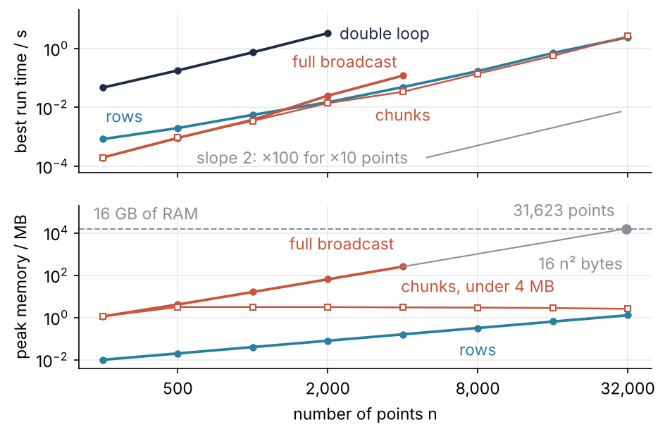
Two panels against the number of points, log-log. Top: best run time of four versions; the double loop lies two orders of magnitude above the three array versions, and all lines rise with a slope close to 2. Bottom: peak memory; the full broadcast grows as 16 n² bytes and would reach 16 GB near 32,000 points, while chunks stay under 4 MB.

This is where we end up. Each point in the top panel is the best of several timeit runs of one version of the code, and each point in the bottom panel is the peak memory tracemalloc recorded during one call. Replacing the inner loop moves the time down by two orders of magnitude, no version changes the slope, and the version without any Python loop pays for it in memory. This page measures how much faster each version is. Why a Python loop is slow in the first place is the subject of a separate tutorial, Why a Python loop is slow and a NumPy array operation is fast (planned).

Setup

Imports, one seeded draw of 32,000 points, of which every smaller set is a prefix, and the style block. The generator is default_rng:

import datetime, json, os, platform, timeit, tracemalloc
import numpy as np
import matplotlib.pyplot as plt

SEED = 20261007
N = 2_000
all_points = np.random.default_rng(SEED).random((32_000, 2))   # uniform in the unit square
points = all_points[:N]
x, y = points[:, 0], points[:, 1]
rho = N / 1.0                          # points per unit area
r_expected = 0.5 / np.sqrt(rho)        # mean nearest-neighbor distance of random points

plt.rcParams.update({
    "figure.figsize": (7, 3.6), "figure.dpi": 110,
    "axes.spines.top": False, "axes.spines.right": False,
    "axes.grid": True, "grid.alpha": 0.25,
    "font.size": 11, "lines.linewidth": 1.8,
})
INK, ACCENT, SECOND, MUTED = "#1f2a44", "#c8553d", "#2a7f9e", "#8a8f98"

print(f"{N} points, density {rho:.0f} per unit area, expected mean distance {r_expected:.5f}")

2000 points, density 2000 per unit area, expected mean distance 0.01118

Step 1: Time the double loop with timeit

The first version everyone writes: for each point, walk through all the others and keep the smallest distance.

def nn_loop(points):
    n = len(points)
    nearest = np.empty(n)
    for i in range(n):
        best = np.inf
        for j in range(n):
            if j != i:
                d = np.sqrt((points[i, 0] - points[j, 0])**2 + (points[i, 1] - points[j, 1])**2)
                if d < best:
                    best = d
        nearest[i] = best
    return nearest

timeit.repeat(func, number=1, repeat=3) calls func once per run, three runs, and returns the three times in seconds. Take the minimum: anything slower than the best run was slowed by the machine, not by your code. timeit wants something to call without arguments; lambda: nn_loop(points) wraps the call, so only the call is timed. %timeit nn_loop(points) in a notebook reports the mean of seven runs instead.

The helper below serves this page, not you: it stores each measurement in timings.json and returns the stored value for a known label, so the page shows the same numbers on every rebuild. On your own code call min(timeit.repeat(...)) directly, or the file hands you old times for new code. It rounds to two significant digits, which is all a timing carries. Run the notebook yourself and the same cells measure your machine.

TIMINGS = "timings.json"
if os.path.exists(TIMINGS):
    with open(TIMINGS) as f:
        timings = json.load(f)
else:
    timings = {"date": str(datetime.date.today()),
               "machine": f"{platform.machine()}, {os.cpu_count()} cores, "
                          f"Python {platform.python_version()}, NumPy {np.__version__}"}

def store(label, value):
    timings[label] = value
    with open(TIMINGS, "w") as f:
        json.dump(timings, f, indent=1)

def best_time(label, func, repeat=5):
    # returns the STORED time if label is in timings.json: delete the file after changing code
    if label not in timings:
        store(label, float(f"{min(timeit.repeat(func, number=1, repeat=repeat)):.2g}"))
    return timings[label]

r_loop = nn_loop(points)
t_loop = best_time("loop 2000", lambda: nn_loop(points), repeat=3)
t_loop_half = best_time("loop 1000", lambda: nn_loop(points[:1_000]), repeat=3)
print(f"measured {timings['date']} on {timings['machine']}")
print(f"double loop, 2,000 points: {t_loop:.2g} s")
print(f"double loop, 1,000 points: {t_loop_half:.2g} s   ratio {t_loop / t_loop_half:.1f}")

r_mean = r_loop.mean()
se = 0.26136 / np.sqrt(N * rho)                         # standard error, Clark and Evans (1954)
r_edge = r_expected + (0.0514 + 0.041 / np.sqrt(N)) * 4 / N   # Donnelly (1978); 4 = perimeter
print(f"mean distance {r_mean:.6f}, expected {r_expected:.6f}, "
      f"R = {r_mean / r_expected:.3f}, standard error {100 * se / r_expected:.1f} %")
print(f"expected with the square's edges {r_edge:.6f} (R = {r_edge / r_expected:.3f}), "
      f"measured mean {(r_mean - r_edge) / se:+.1f} standard errors from it")

measured 2026-10-07 on x86_64, 4 cores, Python 3.12.3, NumPy 2.5.3
double loop, 2,000 points: 3.3 s
double loop, 1,000 points: 0.74 s   ratio 4.5
mean distance 0.011116, expected 0.011180, R = 0.994, standard error 1.2 %
expected with the square's edges 0.011285 (R = 1.009), measured mean -1.3 standard errors from it

Seconds at 2,000 points, and about a quarter of that at 1,000: twice the points, four times the pairs. The mean nearest-neighbor distance is 0.011116 against 0.011180, so R = 0.994. A point near the border has neighbors on one side only, so the edges raise the expected mean to 0.011285 (Donnelly's correction), and the measured mean lies 1.3 standard errors below that. Random points, as drawn.

Step 2: Replace the inner loop by array operations

Subtract a number from an array and NumPy does all the subtractions at once: x - x[i] is an array of 2,000 differences. It replaces the whole inner loop:

def nn_rows(x, y):
    n = len(x)
    d2min = np.empty(n)
    for i in range(n):
        d2 = (x - x[i])**2 + (y - y[i])**2     # squared distances from point i to all points
        d2[i] = np.inf                          # a point is not its own neighbor
        d2min[i] = d2.min()
    return np.sqrt(d2min)

t_rows = best_time("rows 2000", lambda: nn_rows(x, y))
print(f"rows: {t_rows:.2g} s, {t_loop / t_rows:.0f} times faster than the double loop")
print(f"largest difference from the loop: {np.abs(nn_rows(x, y) - r_loop).max()}")

rows: 0.015 s, 220 times faster than the double loop
largest difference from the loop: 0.0

Comparing squared distances and taking one square root per point at the end spares 2,000 square roots per row and changes no answer, because the square root keeps the order. Two orders of magnitude faster, and equal to the loop to the last bit. The loop over a row now runs in compiled code inside NumPy, not in the Python interpreter; the planned tutorial takes that sentence apart.

What it found, in a 0.2 by 0.1 window of the square:

in_window = np.flatnonzero((x > 0.4) & (x < 0.6) & (y > 0.45) & (y < 0.55))
fig, ax = plt.subplots()
for i in in_window:
    d2 = (x - x[i])**2 + (y - y[i])**2
    d2[i] = np.inf
    j = d2.argmin()
    ax.plot([x[i], x[j]], [y[i], y[j]], color=ACCENT, lw=1.2)
ax.plot(x, y, "o", color=INK, ms=4)
ax.set(xlabel="x / side length", ylabel="y / side length", xlim=(0.397, 0.603), ylim=(0.447, 0.553),
       xticks=np.arange(0.40, 0.61, 0.05), yticks=[0.46, 0.50, 0.54], aspect="equal")
plt.show()

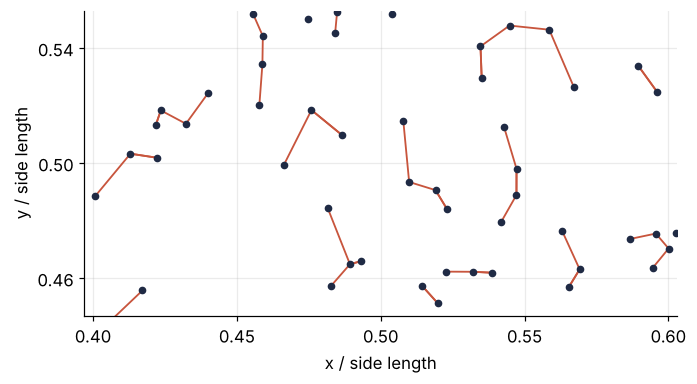
A 0.2 by 0.1 window of the unit square with about forty points as dark dots. A red segment joins each point to its nearest neighbor; most segments are short, a few isolated points reach far.

Most points have a neighbor close by, and a few sit alone, at the end of long segments.

Step 3: Broadcast the whole computation

Removing the loop over the rows needs every pairwise difference at once. When arrays of different shapes meet in arithmetic, NumPy stretches each axis of length 1 to match the other array. On three numbers, with None as an index inserting an axis of length 1:

x3 = np.array([0.0, 0.25, 1.0])
print(x3[:, None].shape, x3[None, :].shape)
print(x3[:, None] - x3[None, :])

(3, 1) (1, 3)
[[ 0.   -0.25 -1.  ]
 [ 0.25  0.   -0.75]
 [ 1.    0.75  0.  ]]

x3[:, None] is a column, x3[None, :] a row, and their difference is the 3 × 3 matrix of all \(x_i - x_j\). That stretching is called broadcasting. The same line on 2,000 points gives a 2,000 × 2,000 matrix, and np.fill_diagonal puts infinity where each point meets itself:

def nn_broadcast(x, y):
    d2 = (x[:, None] - x[None, :])**2 + (y[:, None] - y[None, :])**2   # shape (n, n)
    np.fill_diagonal(d2, np.inf)
    return np.sqrt(d2.min(axis=1))

t_bcast = best_time("broadcast 2000", lambda: nn_broadcast(x, y))
print(f"rows: {t_rows:.2g} s   broadcast: {t_bcast:.2g} s")
print(f"largest difference from the loop: {np.abs(nn_broadcast(x, y) - r_loop).max()}")

rows: 0.015 s   broadcast: 0.025 s
largest difference from the loop: 0.0

Measure memory too, with the standard library's tracemalloc. tracemalloc.start() begins recording every allocation Python makes, and NumPy reports its arrays to it. tracemalloc.get_traced_memory() returns the current and the peak bytes since the start; [1] is the peak, the most memory held at any one moment. tracemalloc.stop() ends the recording. The peak counts the arrays created during the call, not the inputs. A notebook's background threads add a kilobyte or two at random, so the helper stores its result like best_time:

def peak_mb(label, func):
    if label not in timings:
        tracemalloc.start()
        func()
        peak = tracemalloc.get_traced_memory()[1]
        tracemalloc.stop()
        store(label, round(peak / 1e6, 2))
    return timings[label]

m_rows = peak_mb("peak rows 2000", lambda: nn_rows(x, y))
m_bcast = peak_mb("peak broadcast 2000", lambda: nn_broadcast(x, y))
print(f"peak memory   rows: {m_rows:6.2f} MB")
print(f"         broadcast: {m_bcast:6.2f} MB, {m_bcast / m_rows:.0f} times as much")

peak memory   rows:   0.08 MB
         broadcast:  64.13 MB, 802 times as much

Removing the last Python loop did not pay: the same order of magnitude in time as the row version, and 800 times the memory. Two thousand passes of a loop that does real array work are cheap; the full version spends its time moving 64 MB between memory and the processor, not on arithmetic.

Step 4: Find the memory wall

A float64 number takes 8 bytes, so one n × n matrix takes 8 n² bytes:

d2 = (x[:, None] - x[None, :])**2 + (y[:, None] - y[None, :])**2
print(f"one {N} x {N} matrix: {d2.nbytes:,} bytes")

one 2000 x 2000 matrix: 32,000,000 bytes

The peak of 64.13 MB is two of those. While NumPy evaluates the expression it creates temporaries, intermediate arrays it frees as soon as the next operation has used them: the x difference, its square, the y difference, its square, and their sum. Without reuse, the worst moment holds three of them: the x square, the y difference, and the y square being formed, and one step later the two squares and their sum: 24 n² bytes. But when no name refers to a temporary, NumPy squares it in place and adds into it instead of allocating a new array. This reuse is called temporary elision; it needs arrays of at least 256 KiB, and not every platform does it. With it, two remain: the finished x part and the y part. Measure the x part alone and the whole at four sizes:

m = peak_mb("peak x part 2000", lambda: (x[:, None] - x[None, :])**2)
print(f"x part alone, n = 2,000   peak {m:6.2f} MB = {m * 1e6 / (8 * N**2):.2f} matrices")
for n in [150, 1_000, 2_000, 4_000]:          # 150 x 150 numbers are 180 kB, under 256 KiB
    xn, yn = all_points[:n, 0], all_points[:n, 1]
    m = peak_mb(f"peak broadcast {n}", lambda: nn_broadcast(xn, yn))
    print(f"whole, n = {n:5,d}          peak {m:6.2f} MB = {m * 1e6 / (8 * n**2):.2f} matrices")
print(f"by 16 n² bytes: {16 * 20_000**2 / 1e9:.1f} GB at 20,000 points, "
      f"16 GB reached at {np.sqrt(16e9 / 16):,.0f} points, at {np.sqrt(16e9 / 24):,.0f} by 24 n²")

x part alone, n = 2,000   peak  32.13 MB = 1.00 matrices
whole, n =   150          peak   0.54 MB = 3.00 matrices
whole, n = 1,000          peak  16.13 MB = 2.02 matrices
whole, n = 2,000          peak  64.13 MB = 2.00 matrices
whole, n = 4,000          peak 256.00 MB = 2.00 matrices
by 16 n² bytes: 6.4 GB at 20,000 points, 16 GB reached at 31,623 points, at 25,820 by 24 n²

The x part alone peaks at one matrix, so its square was taken in place. The whole peaks at two matrices from 1,000 points on and at three for 150 points, too small for the reuse. Two matrices are 16 n² bytes: 6.4 GB at 20,000 points, and a 16 GB laptop runs out near 32,000, or near 26,000 without the reuse. Past 4,000 points, where the notebook stops, expect a MemoryError, a machine swapping to disk, or a dead kernel.

Step 5: Go around it in chunks

Between one row and all rows lies a block of rows: x[s:e, None] - x[None, :] has shape (e − s, n). The self-distances need a trick. Two integer arrays used as indices are paired element by element, so they pick single entries, not a block:

a = np.zeros((3, 8), dtype=int)
a[np.arange(3), np.arange(5, 8)] = 1     # entries (0, 5), (1, 6), (2, 7)
print(a)

[[0 0 0 0 0 1 0 0]
 [0 0 0 0 0 0 1 0]
 [0 0 0 0 0 0 0 1]]

In a chunk that starts at s, row k is point s + k, whose own distance sits in column s + k; hence the offset:

def nn_chunked(x, y, chunk):
    n = len(x)
    d2min = np.empty(n)
    for s in range(0, n, chunk):
        e = min(s + chunk, n)
        d2 = (x[s:e, None] - x[None, :])**2 + (y[s:e, None] - y[None, :])**2   # shape (e - s, n)
        d2[np.arange(e - s), np.arange(s, e)] = np.inf
        d2min[s:e] = d2.min(axis=1)
    return np.sqrt(d2min)

n = 8_000
x8, y8 = all_points[:n, 0], all_points[:n, 1]
for chunk in [8, 32, 128, 512, 2_048]:
    t = best_time(f"chunked 8000 by {chunk}", lambda: nn_chunked(x8, y8, chunk), repeat=3)
    m = peak_mb(f"peak chunked 8000 by {chunk}", lambda: nn_chunked(x8, y8, chunk))
    print(f"chunk {chunk:5,d}   {t:.2g} s   peak {m:7.2f} MB = {m * 1e6 / (8 * chunk * n):.2f} matrices")

chunk     8   0.14 s   peak    1.60 MB = 3.12 matrices
chunk    32   0.2 s   peak    6.21 MB = 3.03 matrices
chunk   128   0.18 s   peak   24.64 MB = 3.01 matrices
chunk   512   0.33 s   peak   98.37 MB = 3.00 matrices
chunk 2,048   0.48 s   peak  393.28 MB = 3.00 matrices

A chunk of 1 row is Step 2, a chunk of n rows is Step 3, and the chunk size is the knob between them. Larger chunks buy no speed, and past a few hundred rows they cost time as well as memory. The peak holds three matrices of chunk × n numbers, one more than in Step 4, because in the loop d2 holds the previous chunk until the new one is complete. So pick the chunk from a memory budget for the peak:

BUDGET = 4_000_000                      # bytes

def chunk_size(n):
    return max(1, BUDGET // (32 * n))   # 8 bytes x 3 matrices at the peak, plus one spare

for n in [2_000, 8_000, 32_000]:
    xn, yn = all_points[:n, 0], all_points[:n, 1]
    m = peak_mb(f"peak chunked {n}", lambda: nn_chunked(xn, yn, chunk_size(n)))
    print(f"n = {n:6,d}   chunk {chunk_size(n):3d}   peak {m:.2f} MB of a {BUDGET / 1e6:.0f} MB budget")
print(f"largest difference from the loop: {np.abs(nn_chunked(x, y, chunk_size(N)) - r_loop).max()}")

n =  2,000   chunk  62   peak 3.12 MB of a 4 MB budget
n =  8,000   chunk  15   peak 2.95 MB of a 4 MB budget
n = 32,000   chunk   3   peak 2.57 MB of a 4 MB budget
largest difference from the loop: 0.0

The peak stays under the budget at every size. The rule counts four matrices, one more than measured, to leave room for d2min and the result. Without elision a chunk holds about four, which puts the budget at its edge. For your own expression and machine, measure the peak once at a small n and count the matrices.

Step 6: Time every version against the number of points

The sweep runs from 250 to 32,000 points; the double loop stops at 2,000, so that the notebook runs in about a minute, and the full broadcast at 4,000. On log-log axes a slope of 2 means the time grows like n², ten times the points, a hundred times the time, so the cell fits each version's slope over its top three sizes:

sizes = [250, 500, 1_000, 2_000, 4_000, 8_000, 16_000, 32_000]
versions = {   # name: (function of the points, largest n)
    "loop":      (lambda p: nn_loop(p), 2_000),
    "rows":      (lambda p: nn_rows(p[:, 0], p[:, 1]), 32_000),
    "broadcast": (lambda p: nn_broadcast(p[:, 0], p[:, 1]), 4_000),
    "chunked":   (lambda p: nn_chunked(p[:, 0], p[:, 1], chunk_size(len(p))), 32_000),
}
times, peaks = {}, {}
for name, (f, n_max) in versions.items():
    ns = [n for n in sizes if n <= n_max]
    times[name] = np.array([best_time(f"{name} {n}", lambda: f(all_points[:n]),
                                      repeat=3 if name == "loop" or n >= 8_000 else 5) for n in ns])
    if name != "loop":
        peaks[name] = np.array([peak_mb(f"peak {name} {n}", lambda: f(all_points[:n])) for n in ns])

def entry(d, name, k, fmt):
    return format(d[name][k], fmt) if name in d and k < len(d[name]) else ""

print(f"{'':>6s} {'best time / s':^35s}   {'peak memory / MB':^26s}")
print(f"{'n':>6s} {'loop':>8s} {'rows':>8s} {'bcast':>8s} {'chunked':>8s}   {'rows':>8s} {'bcast':>8s} {'chunked':>8s}")
for k, n in enumerate(sizes):
    print(f"{n:6,d} " + " ".join(f"{entry(times, v, k, '.2g'):>8s}" for v in versions)
          + "   " + " ".join(f"{entry(peaks, v, k, '.2f'):>8s}" for v in ["rows", "broadcast", "chunked"]))

slopes = {}
for name in versions:
    ns = sizes[:len(times[name])]
    slopes[name] = np.polyfit(np.log(ns[-3:]), np.log(times[name][-3:]), 1)[0]
print("slope of log time against log n, top three sizes: "
      + ", ".join(f"{v} {s:.1f}" for v, s in slopes.items()))

                  best time / s                   peak memory / MB     
     n     loop     rows    bcast  chunked       rows    bcast  chunked
   250    0.047  0.00084   0.0002   0.0002       0.01     1.13     1.13
   500     0.18    0.002  0.00092  0.00095       0.02     4.13     3.13
 1,000     0.74   0.0056   0.0038   0.0035       0.04    16.13     3.14
 2,000      3.3    0.015    0.025    0.014       0.08    64.13     3.12
 4,000             0.049     0.12    0.034       0.16   256.00     3.01
 8,000              0.17              0.14       0.32              2.95
16,000               0.7              0.56       0.64              2.82
32,000               2.4               2.6       1.28              2.57
slope of log time against log n, top three sizes: loop 2.1, rows 1.9, broadcast 2.5, chunked 2.1

Every slope comes out close to 2, because every version compares all pairs:

labels = {"loop": "double loop", "rows": "rows", "broadcast": "full broadcast", "chunked": "chunks"}
marks = {"loop": dict(color=INK, marker="o"), "rows": dict(color=SECOND, marker="o"),
         "broadcast": dict(color=ACCENT, marker="o"),
         "chunked": dict(color=ACCENT, marker="s", mfc="white", lw=1.2)}
# where each name sits: point index, offset in points, alignment; each label beside its own line
spots_t = {"loop": (-1, (8, 0), "left", "center"), "rows": (0, (2, 9), "left", "bottom"),
           "broadcast": (-1, (-4, 3), "right", "bottom"), "chunked": (4, (0, -9), "center", "top")}
spots_m = {"rows": (5, (0, -8), "center", "top"), "broadcast": (-1, (-6, 9), "right", "bottom"),
           "chunked": (5, (0, 8), "center", "bottom")}

def name_line(ax, d, name, spot, text):
    k, offset, ha, va = spot
    ns = sizes[:len(d[name])]
    ax.annotate(text, (ns[k], d[name][k]), xytext=offset, textcoords="offset points",
                ha=ha, va=va, color=marks[name]["color"])

fig, (ax_t, ax_m) = plt.subplots(2, 1, sharex=True, figsize=(7, 4.4))
for name in versions:
    ns = sizes[:len(times[name])]
    ax_t.plot(ns, times[name], ms=4, **marks[name])
    name_line(ax_t, times, name, spots_t[name], labels[name])
    if name in peaks:
        ax_m.plot(ns, peaks[name], ms=4, **marks[name])
        name_line(ax_m, peaks, name, spots_m[name],
                  "chunks, under 4 MB" if name == "chunked" else labels[name])
n_guide = np.array([5_000, 30_000])
ax_t.plot(n_guide, 2e-4 * (n_guide / 5_000)**2, color=MUTED, lw=1)
ax_t.text(4_200, 2e-4, "slope 2: ×100 for ×10 points", color=MUTED, ha="right", va="center")
ax_t.set(ylabel="best run time / s", xscale="log", yscale="log", ylim=(6e-5, 20))

n_wall = np.sqrt(16e9 / 16)
n_ext = np.geomspace(4_000, n_wall, 50)
ax_m.plot(n_ext, 16 * n_ext**2 / 1e6, color=MUTED, lw=1)
ax_m.text(14_000, 16 * 14_000**2 / 1e6 / 3, "16 n² bytes", color=MUTED, ha="left", va="top")
ax_m.axhline(16_000, color=MUTED, lw=1, ls="--")
ax_m.text(230, 16_000 * 1.8, "16 GB of RAM", color=MUTED, va="bottom")
ax_m.plot(n_wall, 16_000, "o", color=MUTED, ms=6)
ax_m.annotate(f"{n_wall:,.0f} points", (n_wall, 16_000), xytext=(-8, 6), textcoords="offset points",
              ha="right", va="bottom", color=MUTED)
ax_m.set(xlabel="number of points n", ylabel="peak memory / MB", yscale="log", xlim=(200, 40_000),
         ylim=(4e-3, 2e5))
ax_m.set_xticks([500, 2_000, 8_000, 32_000], ["500", "2,000", "8,000", "32,000"])
ax_m.set_xticks([], minor=True)
plt.show()

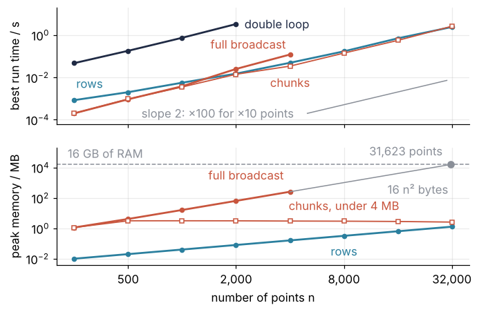
Two panels against the number of points n, log-log. Top: best run time of the double loop, the row version, the full broadcast, and chunks, with a slope-2 guide; the loop lies two orders of magnitude above the rest. Bottom: peak memory; the full broadcast extended by 16 n² bytes reaches the 16 GB line near 32,000 points, chunks stay under 4 MB.

The loop and the array versions run parallel, two orders of magnitude apart. Broadcasting beats the row version up to 1,000 points and loses from 2,000 on, and its memory line reaches 16 GB at the wall of Step 4. Over the row version, chunks buy speed where rows are short: one Python pass per chunk instead of per point makes them several times faster at 250 points, and from 2,000 points on the two run alike. Changing the slope takes another algorithm, such as the KD-tree among the variations.

Pitfalls

The nearest neighbor of a point is itself. Forget the mask and every distance comes out zero. Step 4's matrix has no mask yet:

print(np.sqrt(d2.min(axis=1))[:5], "mean", np.sqrt(d2.min(axis=1)).mean())

[0. 0. 0. 0. 0.] mean 0.0

The diagonal of the matrix, like j == i in the loop, is the distance of each point to itself. np.fill_diagonal(d2, np.inf) fixes the full matrix, d2[i] = np.inf the row version.

Broadcasting over the coordinate axis. The common way to write Step 3 keeps the points as one (n, 2) array:

def nn_broadcast_3d(points):
    diff = points[:, None, :] - points[None, :, :]      # shape (n, n, 2)
    d = np.sqrt((diff**2).sum(axis=-1))
    np.fill_diagonal(d, np.inf)
    return d.min(axis=1)

t_3d = best_time("broadcast 3d 2000", lambda: nn_broadcast_3d(points))
m_3d = peak_mb("peak broadcast 3d 2000", lambda: nn_broadcast_3d(points))
print(f"{t_3d / t_bcast:.1f} times the time of Step 3, peak {m_3d:.2f} MB against {m_bcast:.2f} MB")

5.6 times the time of Step 3, peak 160.00 MB against 64.13 MB

It is several times slower and holds two and a half times the memory. The three-dimensional diff stores two numbers for every pair, twice the size of a distance matrix, and the square and the sum each pass over it once more. Why that costs more time than the memory alone suggests is a question for the planned tutorial. The fix is one change: compute the x and y differences as two separate (n, n) arrays and add their squares, which is Step 3's line.

Trusting one timing. Run the same cell twice and the times differ, and the first call is often the slowest. Other work on the machine and caches warming up are the cause. Take the minimum of several runs, as in Step 1. Under a millisecond, the clock's resolution and the overhead of the call become a visible part of a single run: set number so that each value covers at least 0.2 s, which is what timeit.Timer(f).autorange() picks, and divide each value by number, because it is the total of that many calls.

Variations

scipy.spatial.distance.cdist. Inside the chunk loop, cdist(points[s:e], points) replaces the two broadcast lines and returns distances, not their squares. pdist gives the condensed n(n − 1)/2 distances when you need all of them; the seven-atom cluster uses it.
scipy.spatial.KDTree. KDTree(points).query(points, k=2) returns, in the second column, the nearest neighbor other than the point itself, in n log n time. cKDTree, which older code uses, is its base class and works the same.
A periodic box. For atoms in a simulation box of side 1, wrap the differences with dx -= np.round(dx) before squaring, the minimum image convention. KDTree takes boxsize=1.
The k-th nearest neighbor, or all neighbors within r. Per chunk, after the mask, np.partition(d2, k - 1, axis=1)[:, k - 1] is the squared distance to the k-th nearest neighbor and (d2 < r**2).sum(axis=1) the count within r, the first step toward Ripley's K or the pair correlation function.

Cheat sheet

min(timeit.repeat(lambda: f(a), number=1, repeat=5))  # seconds, best of 5; %timeit f(a): mean of 7 runs
x[:, None] - x[None, :]                         # (n, 1) and (1, n) broadcast to (n, n)
np.fill_diagonal(d2, np.inf)                    # a point is not its own neighbor
np.sqrt(d2.min(axis=1))                         # minimum per row, one sqrt at the end
for s in range(0, n, chunk): e = min(s + chunk, n)   # block of rows x[s:e, None]
chunk = max(1, BUDGET // (32 * n))              # 8 bytes x 3 matrices at the peak + 1 spare; measure yours
tracemalloc.start(); f(a); peak = tracemalloc.get_traced_memory()[1]; tracemalloc.stop()
np.abs(new - old).max()                         # check every faster version against the loop