Random numbers with numpy.random: ten thousand reproducible random walks

The problem: how far does a random walker get?

Ten thousand walkers each take 1,000 steps of +1 or -1, chosen by a fair coin. The walker can be a pollen grain in water, a solute molecule in a solvent, or the free end of a polymer chain; the arithmetic is the same. Theory says that after N steps the mean squared distance from the start is exactly N, here 1,000. It also says how far a simulation may miss: the average over 10,000 walkers is itself a random number, and from one seed to the next it scatters by about 1.41 %. That scatter is the standard error of the mean, and Step 3 derives it. Without it you cannot tell whether a simulated 1,007 agrees with 1,000.

With numpy.random the 10 million coin flips are one call. A simulation that goes into a paper has a second requirement: someone else must be able to run it and get the same numbers, and when it is split across processes, every piece must draw from its own stream.

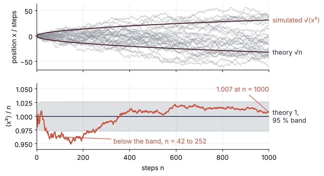
Top: thirty random walks spreading out, with the simulated and the theoretical root mean square distance. Bottom: mean squared displacement of 10,000 walkers divided by the number of steps, against the theory value 1 and its 95 % band; the curve dips below the band between 42 and 252 steps and ends at 1.007.

This is where we end up. The top panel shows thirty of the walks and the root mean square distance, which grows like √n. The bottom panel tests the straight line of diffusion, ⟨x²⟩ = n, by dividing the mean squared displacement of all 10,000 walkers by n: on the line the ratio is 1, and after 1,000 steps it is 1.007. Every walk in it comes from one generator and one seed.

Setup

Imports, the three numbers of the problem, and the style block for the figure:

import numpy as np
import matplotlib.pyplot as plt

W = 10_000         # walkers
N = 1_000          # steps per walker
SEED = 20261006    # the date of the run, fixed before looking at any result

plt.rcParams.update({
    "figure.figsize": (7, 3.6), "figure.dpi": 110,
    "axes.spines.top": False, "axes.spines.right": False,
    "axes.grid": True, "grid.alpha": 0.25,
    "font.size": 11, "lines.linewidth": 1.8,
})
INK, ACCENT, SECOND, MUTED = "#1f2a44", "#c8553d", "#2a7f9e", "#8a8f98"

print(f"{W} walkers x {N} steps, seed {SEED}, NumPy {np.__version__}")

10000 walkers x 1000 steps, seed 20261006, NumPy 2.5.3

Step 1: Create a generator with default_rng and a seed

Random numbers in NumPy come in two layers. At the bottom sits a bit generator, by default PCG64: an engine that turns a seed into a long stream of raw random bits and nothing else. On top sits the Generator that np.random.default_rng(seed) returns, which turns those bits into integers, normal numbers, uniform numbers, and random choices. Two generators from the same seed, and two without one:

a = np.random.default_rng(SEED)
b = np.random.default_rng(SEED)
coins_a = a.integers(0, 2, size=10)
coins_b = b.integers(0, 2, size=10)
print("a:", coins_a)
print("b:", coins_b)
print("same seed, same numbers:", np.array_equal(coins_a, coins_b))

unseeded = [np.random.default_rng().random(10) for _ in range(2)]
print("no seed, same numbers:  ", np.array_equal(*unseeded))
print("bit generator:", type(a.bit_generator).__name__)

rng = np.random.default_rng(SEED)    # the generator every later step draws from

a: [1 1 0 0 1 1 1 0 1 1]
b: [1 1 0 0 1 1 1 0 1 1]
same seed, same numbers: True
no seed, same numbers:   False
bit generator: PCG64

Same seed, same numbers. Without a seed, default_rng pulls fresh entropy from the operating system, so the unseeded generators disagree, and differently on every run. integers excludes the upper bound, so (0, 2) gives 0 or 1: a coin.

How far "the same numbers" reaches depends on the layer. The PCG64 docstring guarantees that a fixed seed always produces the same stream of raw integers. The Generator docstring gives no version compatibility guarantee, because a better algorithm for turning bits into, say, normal numbers may replace the old one. And NumPy's compatibility policy promises identical numbers from a seed only while nothing else changes, neither the NumPy build nor the machine it runs on, since another CPU may round a floating-point edge case differently. So record the NumPy version next to every result; this tutorial keeps it in the header.

If you know np.random.seed and np.random.rand, those are the older interface: one hidden RandomState object shared by the whole program. The Pitfalls say why to leave it.

Step 2: Draw all the steps as one array

A walk is a row of steps, so 10,000 walks are a 10,000 × 1,000 array. Draw it in one call instead of a double loop, and map the coins 0 and 1 to the steps -1 and +1:

steps = 2 * rng.integers(0, 2, size=(W, N), dtype=np.int8) - 1
x = steps.cumsum(axis=1, dtype=np.int16)    # x[:, n - 1] is the position after n steps

print(f"steps {steps.shape} {steps.dtype}, {steps.nbytes / 1e6:.0f} MB")
print(f"x     {x.shape} {x.dtype}")
print("walker 0, first ten steps:", steps[0, :10])
print(f"mean step: {steps.mean():+.5f}")
print("walkers 0 to 4 after N steps:", x[:5, -1])

steps (10000, 1000) int8, 10 MB
x     (10000, 1000) int16
walker 0, first ten steps: [-1 -1 -1  1  1  1  1  1  1 -1]
mean step: +0.00015
walkers 0 to 4 after N steps: [-36 -44 -30 -12 -42]

One row is one walk. cumsum along axis 1 adds up the steps, so the column at index N - 1 holds where each walker stands after 1,000 steps; the first five happen to have all drifted left, by 12 to 44 steps. The mean step is +0.00015, well inside the scatter of the mean of 10 million fair coins, \(1/\sqrt{10^7} = 0.0003\). The dtypes are deliberate: int8 holds a step in one byte and int16 any position up to ±32,767, which keeps the steps at 10 MB.

Step 3: Check the mean squared displacement against theory

Take the final positions, the last column, and cast them to int64 before squaring: a final position near ±1,000 squares to about a million, far beyond int16, and NumPy wraps an integer that overflows without any warning. Their mean square is the mean squared displacement, and its standard error is the standard deviation of the 10,000 squares divided by √W, the scatter of their average (the scipy.stats tutorial uses it throughout). ddof=1 divides by W - 1 instead of W, because the mean inside the standard deviation comes from the same data; it is a spreadsheet's STDEV.S, not STDEV.P.

x_N = x[:, -1].astype(np.int64)
x2 = x_N**2
msd = x2.mean()
rel_se = x2.std(ddof=1) / np.sqrt(W) / msd
rel_se_theory = np.sqrt(2 / W)
z = (msd - N) / (N * rel_se_theory)

print(f"⟨x_N²⟩          = {msd:8.2f}    theory {N}")
print(f"rel. std. error = {100 * rel_se:8.2f} %  theory {100 * rel_se_theory:.2f} %")
print(f"deviation       = {z:+8.2f} theoretical standard errors")

⟨x_N²⟩          =  1007.13    theory 1000
rel. std. error =     1.46 %  theory 1.41 %
deviation       =    +0.50 theoretical standard errors

The theoretical 1.41 % takes four lines. The position \(x_N\) is a sum of N independent steps \(s_i = \pm 1\), each with mean 0 and \(s_i^2 = 1\). Expanding \(\langle x_N^4\rangle\) gives \(N^4\) terms \(\langle s_i s_j s_k s_l\rangle\), and every term in which some index appears an odd number of times averages to zero, because that step is independent and has mean 0. What survives are the terms whose indices pair up: N with all four equal, and \(3N(N-1)\) with two different pairs, since four positions pair up in three ways. So

\[\langle x_N^4\rangle = 3N^2 - 2N, \qquad \operatorname{Var}(x_N^2) = \langle x_N^4\rangle - \langle x_N^2\rangle^2 = 2N^2 - 2N .\]

Divide by W for the variance of the average and by \(N^2\) to make it relative, and the relative standard error is \(\sqrt{2(1 - 1/N)/W}\). The code drops the \(1/N\), which moves the result from 1.4135 % to 1.4142 %.

The simulation lands at 1,007.13, half a theoretical standard error above 1,000. That is agreement. The data's own estimate of the standard error, 1.46 %, is within 4 % of the theory's 1.41 %, so either one gives the same verdict.

Step 4: Swap the step distribution: normal and uniform

The coin is not essential. Draw the steps from a normal distribution with standard deviation 1, or from a uniform distribution on ±√3, whose variance \((\sqrt3)^2/3\) is also 1, and sum each walk:

x_normal = rng.normal(0, 1, size=(W, N)).sum(axis=1)
x_uniform = rng.uniform(-np.sqrt(3), np.sqrt(3), size=(W, N)).sum(axis=1)

for name, final in [("±1", x_N), ("normal", x_normal), ("uniform", x_uniform)]:
    print(f"{name:8s} ⟨x_N²⟩ = {np.mean(final**2):7.1f}")

±1       ⟨x_N²⟩ =  1007.1
normal   ⟨x_N²⟩ =   997.9
uniform  ⟨x_N²⟩ =  1008.3

All three are within one standard error, 14.1, of 1,000. The mean squared displacement depends only on the variance of a single step, which is why the random walk describes diffusion whatever a single collision looks like. Floats have no 8-bit type, so each array of steps takes 80 MB, and because the sum sits on the same line, Python frees that array as soon as the sum is done.

Step 5: Split the run into independent, reproducible streams with SeedSequence.spawn

For a hundred million walkers you split the work into chunks, one per process, and each chunk needs its own stream, independent of the others and reproducible from the run's seed. That is the job of SeedSequence, the object default_rng builds from the seed behind the scenes. It scrambles a seed, however small or regular, into the well-mixed starting state the bit generator needs. spawn(k) derives k children whose states depend only on the parent seed and the child's position, so their streams are independent for any practical purpose, and the whole tree comes back from one number.

Why not default_rng(0), default_rng(1), and so on? Those streams are scrambled too, but they no longer come from the run seed: changing SEED changes nothing, and two experiments that both count from 0 share streams without anyone noticing.

def simulate(seed_seq, walkers):
    """Mean squared displacement after N steps, from a chunk's own generator."""
    rng = np.random.default_rng(seed_seq)
    steps = 2 * rng.integers(0, 2, size=(walkers, N), dtype=np.int8) - 1
    x_N = steps.sum(axis=1, dtype=np.int64)
    return np.mean(x_N**2)

children = np.random.SeedSequence(SEED).spawn(4)
results = [simulate(c, W // 4) for c in children]
print("four chunks:", "  ".join(f"{r:6.1f}" for r in results))
print(f"combined:     {np.mean(results):6.1f}")

four chunks:  956.2  1030.9   960.1  1013.6
combined:      990.2

Each chunk of 2,500 walkers has a standard error of 2.8 %, twice that of the full run, and the four scatter accordingly, the widest 1.5 of their standard errors from 1,000. Combined, they are one run of 10,000 again: 990.2, 0.7 standard errors low. The tree comes back from SEED:

again = [simulate(c, W // 4) for c in np.random.SeedSequence(SEED).spawn(4)]
print("rebuilt from SEED, identical:", np.array_equal(results, again))

rebuilt from SEED, identical: True

To run the chunks in parallel, pool.map(f, items) from the standard library's multiprocessing.Pool calls f once per item, each call in a worker process. functools.partial fills in walkers, so in a script the list comprehension becomes pool.map(partial(simulate, walkers=W // 4), children). Each worker must receive a stream of its own: a child SeedSequence, as here, or one of the generators that rng.spawn(4) returns. Never send one generator to every worker. Each process gets a copy in the same state, and all of them draw the same numbers.

Step 6: Plot the mean squared displacement against the number of steps

The positions from Step 2 hold every intermediate step, so squaring them and averaging each column over walkers gives \(\langle x_n^2\rangle\) for every n at once; the cast to int32 is the overflow guard from Step 3. Theory puts them on the straight line \(\langle x^2\rangle = n\), and its slope is the one-number test. The least-squares slope of a line through the origin is \(\sum n\langle x_n^2\rangle / \sum n^2\), and it should be 1, which with \(\langle x^2\rangle = 2Dt\) and one step per unit of time is a diffusion constant D = 1/2. On a 0 to 1,000 scale a 1 % miss is thinner than the line, so the figure divides by n: the claim becomes the constant 1.

n = np.arange(1, N + 1)
msd_n = (x.astype(np.int32)**2).mean(axis=0)
slope = (n * msd_n).sum() / (n * n).sum()
band = 1.96 * np.sqrt(2 * (n**2 - n) / W)     # 95 % band of the theory, from Step 3
outside = n[np.abs(msd_n - n) > band]

print(f"slope through the origin: {slope:.4f}")
print(f"⟨x²⟩ at n = 100: {msd_n[99]:7.2f}   at n = 1000: {msd_n[-1]:7.2f}")
print(f"outside the 95 % band: {outside.size} of {N} points, n = {outside.min()} to {outside.max()}")

fig, (top, bottom) = plt.subplots(2, 1, sharex=True, figsize=(7, 4.4))
top.plot(n, x[:30].T, color=MUTED, lw=0.7, alpha=0.5)
for sign in (1, -1):
    top.plot(n, sign * np.sqrt(msd_n), color=ACCENT)
    top.plot(n, sign * np.sqrt(n), color=INK, lw=1.2)
top.text(1015, np.sqrt(N), "simulated √⟨x²⟩", color=ACCENT, va="center")
top.text(1015, -np.sqrt(N), "theory √n", color=INK, va="center")
top.set(ylabel="position x / steps")

ratio, rel_band = msd_n / n, band / n
bottom.fill_between(n, 1 - rel_band, 1 + rel_band, color=INK, alpha=0.15, lw=0)
bottom.axhline(1, color=INK, lw=1.2)
bottom.plot(n, ratio, color=ACCENT)
bottom.annotate(f"below the band, n = {outside.min()} to {outside.max()}",
                xy=(100, ratio[99]), xytext=(330, 0.955), color=ACCENT, va="center",
                arrowprops=dict(arrowstyle="-", color=ACCENT, lw=1))
bottom.annotate(f"{ratio[-1]:.3f} at n = {N}", xy=(N, ratio[-1]), xytext=(N, 1.045), ha="right",
                color=ACCENT, arrowprops=dict(arrowstyle="-", color=ACCENT, lw=1))
bottom.text(1015, 1, "theory 1,\n95 % band", color=INK, va="center")
bottom.set(xlabel="steps n", ylabel="⟨x²⟩ / n", xlim=(0, N), ylim=(0.94, 1.06))
plt.show()

slope through the origin: 1.0115
⟨x²⟩ at n = 100:   96.28   at n = 1000: 1007.13
outside the 95 % band: 194 of 1000 points, n = 42 to 252

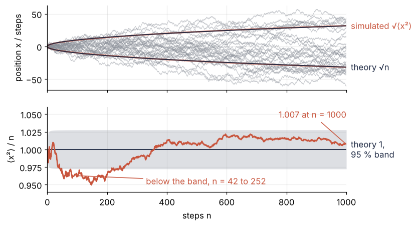
The slope is 1.0115, 1 % too steep, and within its own scatter. The sum weights the large n most, and those points share their walkers, so their errors move together instead of averaging out. The fit therefore scatters nearly as much as the last point alone, 1.41 %.

Between 42 and 252 steps the curve runs below the band, at 0.963 for n = 100, 2.6 standard errors low, and then climbs back. That is one excursion, not 194 failures. The band is pointwise: at any single n, chosen in advance, the curve leaves it in 5 % of seeds. Neighboring points share walkers, so the curve wanders slowly instead of jittering, and over 1,000 steps a slow wander leaves the band somewhere in most seeds. Judge your own simulation at a point or a slope fixed beforehand, as Step 3 did at n = 1,000, not by whether the curve ever leaves the band.

Pitfalls

The legacy global seed. Most code on the web seeds with np.random.seed and draws with np.random.rand. The symptom: the numbers change when someone adds a call that has nothing to do with them. Here a helper adds a little noise to a signal, and calling it once shifts every later number by one place:

def add_noise(signal):
    return signal + 0.01 * np.random.rand()

np.random.seed(SEED)
before = np.random.rand(3)
np.random.seed(SEED)
add_noise(1.0)
after = np.random.rand(3)
with np.printoptions(precision=4):
    print("without the helper:", before)
    print("with the helper:   ", after)

without the helper: [0.8643 0.2309 0.8664]
with the helper:    [0.2309 0.8664 0.1157]

The cause is the hidden RandomState from Step 1, shared by every function in the program, so a draw anywhere moves everyone's stream. np.random.seed seeds only that hidden object, never a generator from default_rng. The fix is one Generator, created once and passed explicitly to every function that draws. Porting old code changes its numbers: RandomState(42) and default_rng(42) give different streams.

One seed reused for runs meant to be independent. Four "independent" runs that each start from default_rng(SEED):

print([float(simulate(SEED, W // 4)) for _ in range(4)])

[1021.0944, 1021.0944, 1021.0944, 1021.0944]

Four identical values, and a standard error computed from their spread would be zero. Spawn the streams as in Step 5. A loop over default_rng(i) makes the values differ, but it loses the run seed, for the reason Step 5 gives.

80 MB of int64 where int8 does. Without dtype, rng.integers returns int64, which would put the steps at 80 MB instead of 10. Going small has two traps of its own: cumsum of an int8 array returns int64 unless you pass dtype, and a small integer that overflows wraps around silently:

print("integers default:", rng.integers(0, 2, size=3).dtype,
      f"-> {np.dtype(np.int64).itemsize * W * N / 1e6:.0f} MB for the steps")
print("cumsum of int8:  ", steps[:1].cumsum(axis=1).dtype)
print("1000² in int16:  ", np.array([1000], dtype=np.int16)**2)

integers default: int64 -> 80 MB for the steps
cumsum of int8:   int64
1000² in int16:   [16960]

The square of 1,000 comes out as 16960, what is left of a million after wrapping modulo 65,536. Step 3 has the cause. Use int8 for steps and int16 for positions, and square in int32 or int64.

Variations

Two or three dimensions. Draw size=(W, N, 2) and sum the squared coordinates; the mean squared distance grows with slope 2, one per dimension.
A biased walk. Steps from 2 * (rng.random((W, N)) < p) - 1 drift by 2p - 1 per step, and the spread around the drift has variance 4p(1 - p)N.
Monte Carlo integration. Points from rng.uniform(-1, 1, size=(M, 2)) land inside the unit circle with probability π/4, and the standard error from Step 3 tells you how many you need (planned tutorial).
Resampling and splits. rng.choice(data, size=(B, n)) draws B bootstrap samples in one call, and rng.permutation(n) shuffles indices for a train and test split.

Cheat sheet

rng = np.random.default_rng(SEED)                 # one Generator, passed to everything that draws
rng.integers(low, high, size, dtype=np.int8)      # high is excluded; default dtype int64
rng.normal(loc, scale, size)                      # Gaussian
rng.uniform(low, high, size)                      # flat on [low, high)
rng.random(size)                                  # flat on [0, 1)
rng.choice(a, size), rng.permutation(n)           # resample, shuffle
rngs = [np.random.default_rng(c) for c in np.random.SeedSequence(SEED).spawn(k)]   # k streams
rngs = rng.spawn(k)                               # the same from an existing generator
# np.random.seed / np.random.rand: legacy global state, do not use in new code