Ray tracing a black hole with solve_ivp: the shadow of M87*

The problem: why M87* has a dark center

In 2019 the Event Horizon Telescope published the first image of a black hole, M87* at the center of the galaxy M87: a bright ring 42 ± 3 microarcseconds (μas) across around a dark center. The dark center is the shadow. Light that passes a black hole of mass M with an impact parameter below \(b_c = \sqrt{27}\,GM/c^2 \approx 5.196\,GM/c^2\) falls in, b being the distance at which the ray would pass the hole if there were no gravity. For M87*, 6.5 × 10⁹ solar masses at 16.8 Mpc, that predicts a dark disk 39.7 μas across.

The path of a light ray past a black hole that does not spin obeys the orbit equation for light,

with r the distance from the hole and φ the angle around it. It is a null geodesic, the path of light, in the Schwarzschild metric of such a hole, written for u with φ as the clock. A planet obeys the same equation with one more term, \(u'' + u = GM/h^2 + 3GMu^2/c^2\), where h is its angular momentum per unit mass. For a particle that moves at the speed of light h grows without bound, and that first term on the right drops out.

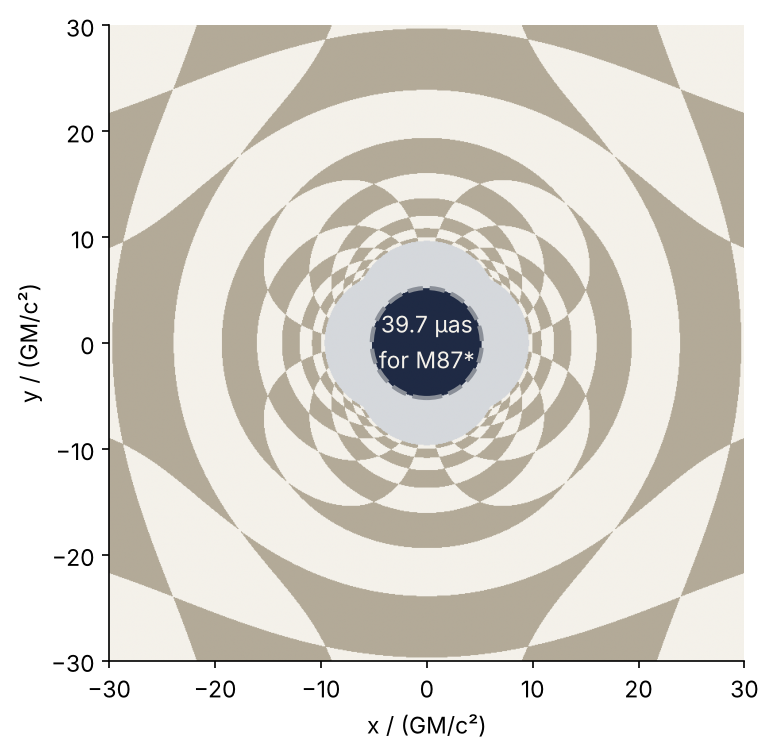
This is where we end up: a checkered wall behind the hole as the hole bends it, with the shadow in the middle and its edge dashed at the b_c you will compute. Each of the 640,000 pixels is one ray, traced backward from the camera toward what it sees; light paths are reversible, so this is the curve the light took. A table of 1,000 solve_ivp calls feeds all of them, because a ray stays in its own plane and only its b matters. On the way you also plot how the deflection runs away as b approaches b_c.

Setup

The code works in units where G = c = M = 1, so a length of 5.2 means 5.2 GM/c², 7.7 km for the Sun. The constants convert to meters and angles: the IAU nominal values for the Sun, and the mass and distance of M87* the EHT used.

import numpy as np
import matplotlib.pyplot as plt
import scipy.constants as const
from matplotlib.colors import to_rgb
from scipy.integrate import solve_ivp

GM_SUN = 1.3271244e20       # m^3/s^2, IAU 2015 nominal
R_SUN = 6.957e8             # m, IAU 2015 nominal
M_M87 = 6.5e9               # solar masses
D_M87 = 16.8                # Mpc
RAD_TO_UAS = np.degrees(1) * 3600 * 1e6

plt.rcParams.update({                      # the look of every figure below
    "figure.figsize": (7.5, 3.5), "figure.dpi": 110,
    "axes.spines.top": False, "axes.spines.right": False,
    "axes.grid": True, "grid.alpha": 0.25,
    "font.size": 11, "lines.linewidth": 1.8,
})
INK, ACCENT, SECOND, MUTED = "#1f2a44", "#c8553d", "#2a7f9e", "#8a8f98"

print(f"GM/c² of the Sun = {GM_SUN / const.c**2:.1f} m")

GM/c² of the Sun = 1476.6 m

Step 1: Write the orbit equation for light as a first-order system

With \(w = du/d\varphi\) the orbit equation becomes two first-order equations, \(u' = w\) and \(w' = 3u^2 - u\), in units of GM/c². The independent variable is φ, not time and not r. φ grows steadily along every ray, also through the closest approach, where r turns around and stops being a usable clock.

A ray starts at the camera, far away, so u = 0. Without the hole it would be the straight line \(r\sin\varphi = b\), that is \(u = \sin\varphi / b\), whose slope at φ = 0 is \(w = 1/b\). That is the start state, and from there the ray is followed past the hole, backward along the path the light took. Run two rays over one full turn in φ and look at where each one ends:

def light(phi, y):
    u, w = y
    return [w, 3 * u**2 - u]

for b in [8, 4]:
    sol = solve_ivp(light, (0, 2 * np.pi), [0.0, 1 / b])
    print(f"b = {b}: u = {sol.y[0, -1]:.3g} at phi = {sol.t[-1]:.2f}, status {sol.status}")
    print(f"       {sol.message}")

b = 8: u = -0.0582 at phi = 6.28, status 0
       The solver successfully reached the end of the integration interval.
b = 4: u = 3.86e+27 at phi = 5.08, status -1
       Required step size is less than spacing between numbers.

Neither is a ray. At b = 8 the light passed the hole and went back out to u = 0, but nothing told the solver to stop there, so it carried on to u = −0.058, a negative radius. At b = 4 the light fell toward r = 0, u grew to 3.9 × 10²⁷, and the solver gave up with status −1. Both rays need a stop.

Step 2: Stop each ray at the horizon or at escape with events

Two terminal events give each ray its stop, as in solve_ivp from the ground up, Step 5. The horizon is the sphere r = 2 GM/c², u = 1/2, inside which nothing, light included, comes back out; the event horizon returns u − 1/2 and fires on the way in. The event escape returns u and fires only when u falls through zero, so the start at u = 0, where u rises, does not trigger it.

Which list in sol.t_events is non-empty tells the fate. For an escaping ray it also gives the deflection. The straight line u = sin φ / b returns to u = 0 at φ = π, so whatever φ the ray needs beyond π is the bending, α = φ_end − π.

def horizon(phi, y):
    return y[0] - 0.5
horizon.terminal, horizon.direction = True, 1

def escape(phi, y):
    return y[0]
escape.terminal, escape.direction = True, -1

def trace(b, rtol=1e-10, atol=1e-12, **kwargs):
    """Fate of the ray with impact parameter b: ("captured", phi) or ("escaped", alpha), and the solution."""
    sol = solve_ivp(light, (0, 40 * np.pi), [0.0, 1 / b], events=[horizon, escape],
                    rtol=rtol, atol=atol, **kwargs)
    if sol.t_events[0].size:
        return "captured", sol.t_events[0][0], sol
    return "escaped", sol.t_events[1][0] - np.pi, sol

for b in [4, 6, 8]:
    fate, angle, sol = trace(b)
    if fate == "captured":
        print(f"b = {b}: captured at phi = {angle:.2f} rad")
    else:
        print(f"b = {b}: escaped, bent by {np.degrees(angle):.1f}°")

b = 4: captured at phi = 2.54 rad
b = 6: escaped, bent by 98.5°
b = 8: escaped, bent by 49.2°

The span of 40π is only an upper bound; every ray ends at an event long before it. At b = 8 the light is bent by 49.2°, at b = 6 by 98.5°, and somewhere between 6 and 4 the hole stops letting go.

Step 3: Find the critical impact parameter by bisection

The ray at b = 5 is captured and the one at b = 6 escapes, so the edge of the shadow is in between. Halve the interval, keep the half where the fate changes, and repeat. Forty halvings shrink it to 10⁻¹². A plain loop does this; a root finder wants a continuous function, and the fate jumps from one outcome to the other.

b_lo, b_hi = 5.0, 6.0                      # captured, escaped
for _ in range(40):
    b_mid = 0.5 * (b_lo + b_hi)
    if trace(b_mid)[0] == "captured":
        b_lo = b_mid
    else:
        b_hi = b_mid
b_c = 0.5 * (b_lo + b_hi)
print(f"b_c = {b_c:.7f}   sqrt(27) = {np.sqrt(27):.7f}")

fate, alpha, sol = trace(5.1962, dense_output=True)
phi = np.linspace(0, sol.t[-1], 20_000)
r_min = 1 / sol.sol(phi)[0].max()
print(f"b = 5.1962: {fate}, closest approach r = {r_min:.3f}, bent by {np.degrees(alpha):.0f}°,"
      f" {sol.nfev} function calls")

b_c = 5.1961524   sqrt(27) = 5.1961524
b = 5.1962: escaped, closest approach r = 3.007, bent by 642°, 1712 function calls

Eight digits of agreement with √27. The ray that starts 5 × 10⁻⁵ above b_c comes within 3.007 GM/c² of the hole and is bent by 642°: it sweeps more than two full turns, nearly all of them close to r = 3 GM/c². That radius is the photon sphere, where light can circle the hole, but not for long. Put u = 1/3 + δ into the equation and the offset obeys δ'' = δ, so it grows by a factor e with every radian of φ. A ray that starts a factor e closer to b_c stays one radian longer, and the deflection grows like −log(b − b_c) without bound.

Step 4: Check the weak field and convert to angles on the sky

Far from the hole the deflection must approach Einstein's 4GM/(c²b), which is 4/b in our units:

for b in [20, 100, 1e3, 1e4]:
    alpha = trace(b)[1]
    print(f"b = {b:6.0f}:  alpha = {np.degrees(alpha):8.5f}°   4/b = {np.degrees(4 / b):8.5f}°"
          f"   excess {alpha / (4 / b) - 1:6.2%}")

theta_g = GM_SUN * M_M87 / const.c**2 / (D_M87 * 1e6 * const.parsec) * RAD_TO_UAS
print(f"M87*: 1 GM/c² = {theta_g:.2f} μas on the sky, shadow 2 b_c = {2 * b_c * theta_g:.1f} μas")

b =     20:  alpha = 13.52960°   4/b = 11.45916°   excess 18.07%
b =    100:  alpha =  2.36188°   4/b =  2.29183°   excess  3.06%
b =   1000:  alpha =  0.22986°   4/b =  0.22918°   excess  0.30%
b =  10000:  alpha =  0.02292°   4/b =  0.02292°   excess  0.03%
M87*: 1 GM/c² = 3.82 μas on the sky, shadow 2 b_c = 39.7 μas

The excess falls from 18 % at b = 20 to 0.03 % at b = 10⁴, tenfold for every factor of ten in b. That is the next term of the weak-field series, 15π/(4b²) (Keeton and Petters, Phys. Rev. D 72, 104006, 2005), which the integration reproduces without being told.

For M87*, one GM/c² seen from 16.8 Mpc is 3.82 μas, and the shadow is 39.7 μas across. The EHT measured 42 ± 3 μas, but what it sees is the glowing gas just outside the shadow's edge, so the ring comes out somewhat larger than the edge itself.

Step 5: Tabulate the deflection once and plot it

Every pixel needs α(b), and the ray of Step 3 alone took 1,712 function calls. Compute a table once and interpolate. Because α grows like −log(b − b_c), 600 of the values crowd toward b_c on a logarithmic grid and 400 cover the rest out to b = 60. The loop takes about 20 s. The last lines check the table against a direct trace at b = 8, and say how far the difference moves the ray's landing point on the wall that Step 6 paints, 100 GM/c² behind the hole.

b_table = np.concatenate([b_c + np.geomspace(1e-6, 1, 600), np.linspace(b_c + 1, 60, 401)[1:]])
alpha_table = np.array([trace(b)[1] for b in b_table])

print(f"{b_table.size} rays, alpha from {np.degrees(alpha_table[0]):.0f}° to {np.degrees(alpha_table[-1]):.2f}°")
for d in [1e-6, 1e-5, 1e-4]:
    print(f"b - b_c = {d:.0e}:  alpha = {np.degrees(np.interp(b_c + d, b_table, alpha_table)):.0f}°")
a_table, a_trace = np.interp(8, b_table, alpha_table), trace(8)[1]
wall_hit = lambda a: (8 - 100 * np.sin(a)) / np.cos(a)     # landing height on that wall, derived in Step 6
print(f"b = 8:  table {np.degrees(a_table):.3f}°   trace {np.degrees(a_trace):.3f}°"
      f"   hit moves by {abs(wall_hit(a_table) - wall_hit(a_trace)):.3f} GM/c²")

1000 rays, alpha from 863° to 4.02°
b - b_c = 1e-06:  alpha = 863°
b - b_c = 1e-05:  alpha = 731°
b - b_c = 1e-04:  alpha = 599°
b = 8:  table 49.214°   trace 49.202°   hit moves by 0.048 GM/c²

Each factor of ten closer to b_c adds 132°, which is ln 10 radians, the growth by e per radian of Step 3. Interpolation at b = 8 is off by 0.012°, which moves the landing point by 0.048 GM/c², a two-hundredth of the wall's 10 GM/c² squares.

Show code

Copy

b_weak = np.linspace(b_c, 30, 300)
fig, ax = plt.subplots()
ax.plot(b_table, np.degrees(alpha_table), color=ACCENT)
ax.plot(b_weak, np.degrees(4 / b_weak), color=SECOND, lw=1.1)
ax.axvline(b_c, color=MUTED, ls="--", lw=1)
ax.text(b_c - 0.4, 370, f"b_c = {b_c:.3f}", color=MUTED, ha="right")
ax.text(17, 40, "Einstein 4GM/(c²b)", color=SECOND)
ax.text(6.6, 150, "solve_ivp", color=ACCENT)
ax.set(xlabel="b / (GM/c²)", ylabel="α / degrees", xlim=(0, 30), ylim=(0, 400))
plt.show()

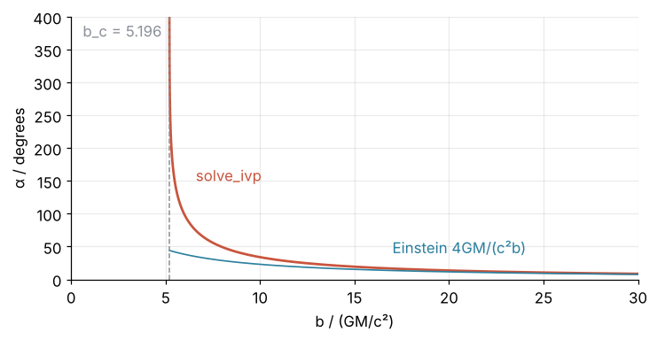
Beyond b ≈ 20 the two curves are hard to tell apart. Inside it the computed deflection pulls away from 4/b and runs off to infinity at the dashed b_c.

Step 6: Render the lensed image

The camera is far away, as for M87*, so a pixel at distance b and azimuth ψ from the image center sees along the ray with impact parameter b in the plane at that ψ. A wall 120 GM/c² square, checkered in squares of 10 with one centered on the line of sight, stands L = 100 GM/c² behind the hole.

The orbit is symmetric about its closest approach, so the outgoing straight line passes the hole at the same distance b, turned by α. It crosses the wall at signed height R = (b − L sin α)/cos α, as this ray at b = 12 shows:

Show code

Copy

L_wall = 100.0
fate, alpha12, sol = trace(12.0, dense_output=True)
phi = np.linspace(1e-3, sol.t[-1] - 1e-3, 2000)
r = 1 / sol.sol(phi)[0]
z, y = -r * np.cos(phi), r * np.sin(phi)            # camera at z = -infinity, wall at z = +L
keep = (z > -40) & (z < L_wall)
hit = (12 - L_wall * np.sin(alpha12)) / np.cos(alpha12)

fig, ax = plt.subplots()
ax.add_patch(plt.Circle((0, 0), 2, color=INK))
ax.plot([-40, 30], [12, 12], color=MUTED, ls="--", lw=1)          # incoming asymptote, run past the hole
z_out = np.array([-25, L_wall])
ax.plot(z_out, 12 / np.cos(alpha12) - np.tan(alpha12) * z_out, color=MUTED, ls="--", lw=1)   # outgoing
for foot in [(0, 12), (12 * np.sin(alpha12), 12 * np.cos(alpha12))]:
    ax.plot([0, foot[0]], [0, foot[1]], color=MUTED, lw=1)
ax.text(-1.2, 6, "b", color=MUTED, ha="right", va="center")
ax.text(3.6, 4.5, "b", color=MUTED, ha="left", va="center")
ax.plot(z[keep], y[keep], color=ACCENT, zorder=3)
ax.axvline(L_wall, color=INK, lw=1.2)
ax.plot(L_wall, hit, "o", color=ACCENT, ms=6, zorder=4)
ax.text(L_wall - 2, hit - 3, f"{hit:.1f}".replace("-", "−"), color=ACCENT, ha="right", va="top")
ax.text(L_wall - 3, 18, "wall", color=INK, ha="right")
ax.set(xlabel="z / (GM/c²)", ylabel="y / (GM/c²)", xlim=(-40, 110), ylim=(-45, 25), aspect="equal")
plt.show()
print(f"b = 12: bent by {np.degrees(alpha12):.1f}°, lands at y = {hit:.1f} on the wall")

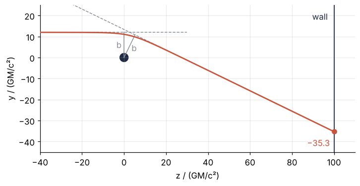
b = 12: bent by 25.9°, lands at y = -35.3 on the wall

It bends by 25.9° and lands at R = −35.3, across the axis. The pixel keeps its azimuth, so it shows the wall point R(cos ψ, sin ψ), and a negative R puts it on the opposite side of the center. Rays bent by 90° or more never reach the wall (cos α passes zero); their pixels are pale, like those of rays that miss its edge.

The point behind the hole, R = 0, is seen at every ψ: a ring. That is the Einstein ring, at the b where b − L sin α changes sign:

Copy

n = 800
x = np.linspace(-30, 30, n)
X, Y = np.meshgrid(x, x)
b_pix = np.hypot(X, Y)
psi = np.arctan2(Y, X)
alpha_pix = np.interp(b_pix, b_table, alpha_table)
R = (b_pix - L_wall * np.sin(alpha_pix)) / np.cos(alpha_pix)    # signed radius on the wall
WX, WY = R * np.cos(psi), R * np.sin(psi)

shadow = b_pix < b_c
pale = (alpha_pix >= np.pi / 2) | (np.abs(WX) > 60) | (np.abs(WY) > 60)
tile = (np.floor(WX / 10 + 0.5) + np.floor(WY / 10 + 0.5)) % 2 == 1

def paint(shadow_color, tile_colors, pale_color):
    rgb = np.where(tile[..., None], to_rgb(tile_colors[1]), to_rgb(tile_colors[0]))
    rgb[pale] = to_rgb(pale_color)
    rgb[shadow] = to_rgb(shadow_color)
    return rgb

outer = b_table > 10
g = b_table[outer] - L_wall * np.sin(alpha_table[outer])
i = np.flatnonzero(np.diff(np.sign(g)))[0]
b_ring = np.interp(0, g[i:i + 2], b_table[outer][i:i + 2])
print(f"Einstein ring at b = {b_ring:.1f} GM/c²")

fig, ax = plt.subplots(figsize=(5.5, 5.5))
ax.imshow(paint(INK, ["#f4f1ea", "#b3aa98"], "#d5d8dc"), origin="lower", extent=(-30, 30, -30, 30))
ax.add_patch(plt.Circle((0, 0), b_c, fill=False, color=MUTED, ls="--", lw=2))   # b_c, as in Step 5
ax.text(0, 0, f"{2 * b_c * theta_g:.1f} μas\nfor M87*", color="#f4f1ea", ha="center", va="center",
        linespacing=1.2)                   # inside the shadow, where it hides no part of the image
ax.set(xlabel="x / (GM/c²)", ylabel="y / (GM/c²)")
ax.grid(False)
plt.show()

Einstein ring at b = 21.5 GM/c²

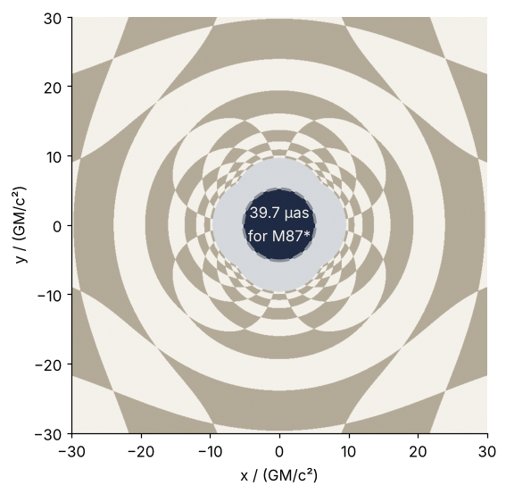
With α ≈ 4/b from Step 4 and sin α ≈ α, b − 4L/b = 0 gives b = 2√L = 20. The computed ring sits at 21.5, because near b = 20 the deflection is 18 % above 4/b. Inside the ring R is negative, so you see the same face of the wall again, turned by 180° and squeezed toward the shadow. The camera at infinity and the straight asymptote make this a model, not a picture of M87*; b_c and the 39.7 μas do not depend on the wall.

Pitfalls

Default tolerances near the critical ray. A ray close to b_c spends many radians near u = 1/3, and the error of each step adds up turn after turn:

for rtol, atol in [(1e-3, 1e-6), (1e-10, 1e-12)]:
    fate, alpha, sol = trace(5.1962, rtol=rtol, atol=atol)
    print(f"rtol={rtol:<6g} atol={atol:<6g}  bent by {np.degrees(alpha):4.0f}°   nfev = {sol.nfev:5d}")

rtol=0.001  atol=1e-06   bent by  416°   nfev =    86
rtol=1e-10  atol=1e-12   bent by  642°   nfev =  1712

With the defaults the ray is bent by 416° instead of 642°, after 86 function calls instead of 1,712, and a bisection built on them inherits the error. Use rtol=1e-10, atol=1e-12, and check that b_c does not move when both are ten times tighter.

An absolute tolerance above the state, far from the hole. At the limb of the Sun, b = R☉c²/GM☉ = 4.7 × 10⁵, the tolerances that serve every other ray give 1.691″ instead of Einstein's 1.75″:

b_sun = R_SUN * const.c**2 / GM_SUN
for atol in [1e-12, 1e-18]:
    alpha = trace(b_sun, atol=atol)[1]
    print(f"atol={atol:g}:  bent by {np.degrees(alpha) * 3600:.4f} arcsec")

atol=1e-12:  bent by 1.6913 arcsec
atol=1e-18:  bent by 1.7512 arcsec

There u is at most 2 × 10⁻⁶, and the part of it that carries the bending, driven by the 3u² term and so of order 1/b² = 4.5 × 10⁻¹², is barely above atol = 1e-12. The error control lets it slide. Put atol far below the smallest value of the state you care about, as solve_ivp from the ground up says in Step 4; 1e-18 gives 1.7512″.

The image's angular scale. The size of the shadow is a ratio of two lengths, and the two usual slips give numbers that look like answers:

GM_m = GM_SUN * M_M87 / const.c**2                         # meters
for slip, size in [("D in parsecs", 2 * b_c * GM_m / (D_M87 * 1e6)),
                   ("no RAD_TO_UAS", 2 * b_c * GM_m / (D_M87 * 1e6 * const.parsec)),
                   ("correct", 2 * b_c * GM_m / (D_M87 * 1e6 * const.parsec) * RAD_TO_UAS)]:
    print(f"{slip:14s} {size:.3g}")

D in parsecs   5.94e+06
no RAD_TO_UAS  1.92e-10
correct        39.7

GM/c² in meters over the distance in parsecs gives 5.9 × 10⁶, millions of radians for something on the sky. Forgetting the factor from radians to microarcseconds gives 1.92 × 10⁻¹⁰, which reads as a shadow no telescope could ever resolve. Convert both lengths to meters before dividing, and compare with the 3.82 μas per GM/c² of Step 4.

Variations

• A glowing thin disk. Replace the wall by a disk in the equatorial plane, as Luminet drew it in 1979. The disk cuts each ray's plane along a line through the hole, and an event at the φ of that line gives where the ray meets the disk.
• The secondary images. Rays bent by 270° to 450° come around and reach the wall a second time. Zoom the grid to within about 0.03 GM/c² of b_c and make the table denser there.
• Mercury's perihelion. Add GM/h² back to the right-hand side for a planet; an event on du/dφ = 0 with direction = -1 gives the angle of each perihelion, and their drift per orbit is the precession (planned as a Recipe on this site).
• A spinning black hole. A ray no longer stays in one plane, so the table in b no longer works: trace one ray per pixel with the Kerr null geodesic equations in r and θ, each in second-order form so that it passes its turning points as u does here. The spin a is the one new parameter; the shadow shifts and flattens on one side.

Cheat sheet

light = lambda phi, y: [y[1], 3 * y[0]**2 - y[0]]   # u = 1/r, units GM/c^2
y0 = [0.0, 1 / b]                                   # from the camera, far away
horizon = lambda phi, y: y[0] - 0.5                 # r = 2: captured; terminal, direction = 1
escape = lambda phi, y: y[0]                        # u = 0 again: escaped; terminal, direction = -1
sol = solve_ivp(light, (0, 40 * np.pi), y0, events=[horizon, escape], rtol=1e-10, atol=1e-12)
alpha = sol.t_events[1][0] - np.pi                  # deflection, if t_events[1] is non-empty
alpha_pix = np.interp(b_pix, b_table, alpha_table)  # one table, every pixel
R = (b - L * np.sin(alpha)) / np.cos(alpha)         # where the ray hits a wall at distance L
size = 2 * b_c * GM / (c**2 * D)                    # shadow in radians, GM/c^2 and D in meters

Further reading

• scipy.integrate.solve_ivp reference, in particular the events parameter.
• Event Horizon Telescope Collaboration, ApJL 875, L1 (2019), the image, and paper VI, ApJL 875, L6, for the mass from the size of the ring.
• J.-P. Luminet, "Image of a spherical black hole with thin accretion disk", A&A 75, 228 (1979), the first picture of a black hole with a disk.
• J. B. Hartle, Gravity: An Introduction to Einstein's General Relativity (Addison-Wesley, 2003), chapter 9, for the orbit equation and the deflection of light.
• Related on this site: solve_ivp from the ground up: the pendulum beyond small angles for events and tolerances, Stiffness: why an explicit solver crawls on a reaction that has long settled, Draw a phase portrait of a two-variable ODE system. Planned: Mercury's perihelion precession as a Recipe, and this tutorial in Julia.
• Download the notebook. It was executed with the library versions in the header.