The Sievert integral with scipy.integrate.quad: dose beside a shielded pipe

The problem: how much dose reaches a worker beside a shielded pipe?

A 2 m pipe carries cooling water with cobalt-60 in it, 1 MBq per meter of pipe: a million decays per second in every meter. A worker stands 1 m from the middle of the pipe, behind a 10 cm concrete wall that runs parallel to it. The quick estimate lumps the 2 MBq into a point at the pipe's center and gives 161 nGy/h. Keeping the pipe a pipe leads to the Sievert integral, which has no closed form and which quad evaluates for you (Numerical integration with scipy.integrate covers the function itself). It gives 109 nGy/h. The point estimate is 48 % high.

That number counts only uncollided photons, those that cross the wall without interacting with it. Photons that scatter in the concrete and still reach the worker arrive on top, so everything below is a lower bound, and the first pitfall comes back to it. The quantity is the air kerma rate: the energy the photons hand to charged particles per kilogram of air, in gray per hour, the standard measure of a photon dose rate in air. Step 4 turns photon counts into it.

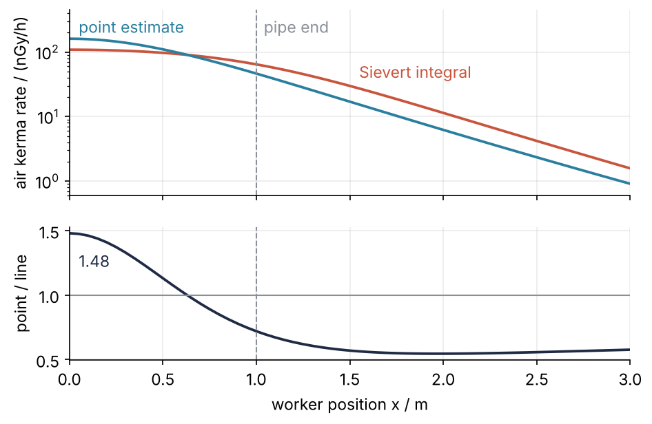
Two panels against the worker's position along the wall, 0 to 3 m. Top: air kerma rate in nGy/h on a log scale, Sievert integral and point estimate, 109 against 161 at the middle. Bottom: their ratio, 1.48 at the middle, below 1 from about 0.6 m on, before the pipe's end at 1 m.

Walk along the wall and the error changes sign. In front of the middle the point estimate is too high; past the end of the pipe it is too low, by almost a factor of two. Each curve is 61 positions of the worker, and every position of the line curve costs four calls to quad. Step 5 draws it.

Setup

All lengths are in centimeters, because the attenuation tables are. The table rows are typed in from the NIST tables, three energies that bracket the two photon energies cobalt-60 emits, its gamma lines.

import numpy as np
import matplotlib.pyplot as plt
from scipy.integrate import quad

plt.rcParams.update({
    "figure.figsize": (7, 3.6), "figure.dpi": 110,
    "axes.spines.top": False, "axes.spines.right": False,
    "axes.grid": True, "grid.alpha": 0.25,
    "font.size": 11, "lines.linewidth": 1.8,
})
INK, ACCENT, SECOND, MUTED = "#1f2a44", "#c8553d", "#2a7f9e", "#8a8f98"

L = 200.0                # pipe length, cm
h = 100.0                # distance from pipe to worker, cm
t = 10.0                 # wall thickness, cm
S_L = 1e6 / 100          # 1 MBq per m of pipe, in Bq/cm

E = np.array([1.1732, 1.3325])        # Co-60 gamma lines, MeV (NNDC)
Y = np.array([0.9985, 0.9998])        # photons per decay

# NIST X-ray mass attenuation coefficients (Hubbell and Seltzer, NISTIR 5632)
table_E = np.array([1.0, 1.25, 1.5])                     # MeV
concrete_mu_rho = np.array([0.06495, 0.05807, 0.05288])  # cm²/g, ordinary concrete
rho_concrete = 2.3                                       # g/cm³
air_muen_rho = np.array([0.02789, 0.02666, 0.02547])     # cm²/g, dry air

print(f"pipe {L:.0f} cm, worker at {h:.0f} cm, wall {t:.0f} cm, source {S_L:.0f} Bq/cm")

pipe 200 cm, worker at 100 cm, wall 10 cm, source 10000 Bq/cm

Step 1: Look up the attenuation coefficient and count mean free paths

A beam of photons that crosses a thickness \(t\) of material keeps a fraction \(e^{-\mu t}\) of its uncollided photons. The linear attenuation coefficient \(\mu\) is the probability per centimeter that a photon interacts in any way that takes it out of the beam, absorbed or scattered aside. Its inverse is the mean free path, so \(b = \mu t\) counts how many mean free paths thick the wall is.

You do not compute \(\mu\); you look it up. The NIST tables of X-ray mass attenuation coefficients by Hubbell and Seltzer list \(\mu/\rho\) for the elements from hydrogen to uranium and for 48 compounds and mixtures, ordinary concrete and air among them, and NIST's XCOM program gives it for any composition you type in. Multiply by the density and you have \(\mu\). The tables sit on a fixed energy grid, and between grid points the coefficients follow power laws closely, so interpolate in the logarithms of both energy and coefficient:

def loglog_interp(E, table_E, table_val):
    return np.exp(np.interp(np.log(E), np.log(table_E), np.log(table_val)))

mu_rho = loglog_interp(E, table_E, concrete_mu_rho)
mu = mu_rho * rho_concrete            # 1/cm
b = mu * t                            # mean free paths across the wall

for Ei, mr, mui, bi in zip(E, mu_rho, mu, b):
    print(f"E = {Ei:.4f} MeV   mu/rho = {mr:.4f} cm²/g   mu = {mui:.4f} /cm"
          f"   b = {bi:.2f}   exp(-b) = {np.exp(-bi):.3f}")

E = 1.1732 MeV   mu/rho = 0.0599 cm²/g   mu = 0.1379 /cm   b = 1.38   exp(-b) = 0.252
E = 1.3325 MeV   mu/rho = 0.0562 cm²/g   mu = 0.1292 /cm   b = 1.29   exp(-b) = 0.275

The wall is 1.38 mean free paths thick at the lower energy and 1.29 at the upper one. Straight through it, about a quarter of the photons survive uncollided, slightly more of the harder photons.

Step 2: Follow a slanted ray: the point-source estimate

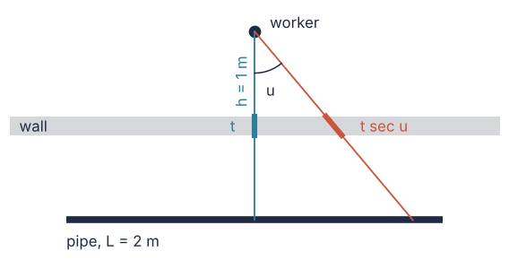
Only the ray along the perpendicular crosses the wall along its thickness \(t\). A ray that leaves the pipe at an angle \(u\) from the perpendicular runs through the concrete along \(t/\cos u = t \sec u\) and keeps \(e^{-b \sec u}\) of its photons. The parts of the pipe far from the worker are therefore dimmer than the inverse-square law alone says. Where the wall stands between pipe and worker does not matter, only its thickness and the angle.

Show code

fig, ax = plt.subplots(figsize=(7, 3.4))
wall = (0.45, 0.55)                                  # to scale: h = 1 m, t = 10 cm
ax.axhspan(*wall, color=MUTED, alpha=0.35, lw=0)
ax.plot([-1, 1], [0, 0], color=INK, lw=5, solid_capstyle="butt")
ax.plot(0, 1, "o", color=INK, ms=8)
ax.plot([0, 0], [0, 1], color=SECOND, lw=1.2)
ax.plot([0, 0], wall, color=SECOND, lw=4)               # the straight path inside the wall
u = np.radians(40)
x_el = np.tan(u)                                     # pipe element seen at angle u
ax.plot([x_el, 0], [0, 1], color=ACCENT, lw=1.2)
ys = np.array(wall)
ax.plot(x_el * (1 - ys), ys, color=ACCENT, lw=4)     # the slanted path inside the wall
arc = np.linspace(-np.pi / 2, -np.pi / 2 + u, 30)
ax.plot(0.22 * np.cos(arc), 1 + 0.22 * np.sin(arc), color=INK, lw=1)
ax.text(0.06, 0.66, "u", color=INK)
ax.text(-0.13, 0.47, "t", color=SECOND)
ax.text(0.56, 0.47, "t sec u", color=ACCENT)
ax.text(0.08, 1.02, "worker", color=INK)
ax.text(-1, -0.14, "pipe, L = 2 m", color=INK)
ax.text(-1.25, 0.47, "wall", color=INK)
ax.text(-0.12, 0.62, "h = 1 m", color=SECOND, rotation=90)
ax.set(xlim=(-1.3, 1.3), ylim=(-0.25, 1.12), aspect="equal")
ax.set_axis_off()
plt.show()

Top view of the pipe, the concrete wall, and the worker 1 m away. The perpendicular ray crosses the wall along its thickness t; a ray from further along the pipe, at angle u, crosses it along the longer path t sec u.

The shortcut puts all \(S_L L\) becquerels at the pipe's center, at distance \(r = \sqrt{h^2 + x^2}\) from a worker who has walked a distance \(x\) along the wall. Its one ray has \(\sec u = r/h\):

def fluence_point(x):
    """Uncollided photons per cm² per s, whole pipe lumped at its center."""
    r = np.hypot(h, x)
    return S_L * L * Y / (4 * np.pi * r**2) * np.exp(-b * r / h)

phi_point = fluence_point(0.0)
for Ei, p in zip(E, phi_point):
    print(f"E = {Ei:.4f} MeV   point estimate {p:.2f} photons/(cm² s)")

E = 1.1732 MeV   point estimate 4.00 photons/(cm² s)
E = 1.3325 MeV   point estimate 4.37 photons/(cm² s)

In front of the middle that ray goes straight through: 4.00 and 4.37 photons per square centimeter per second, the numbers the pipe has to beat.

Step 3: Sum the pipe into the Sievert integral with quad

Cut the pipe into elements \(dx\), each a point source of strength \(S_L\,dx\). An element at distance \(r\), seen under the angle \(u\), contributes \(S_L\,dx\,e^{-b\sec u}/(4\pi r^2)\). Measure its position from the foot of the perpendicular, \(x = h\tan u\), and the inverse square and the length element combine into the angle alone:

\[\frac{dx}{r^2} = \frac{h\sec^2 u\,du}{h^2\sec^2 u} = \frac{du}{h}.\]

The whole pipe is then

\[\varphi = \frac{S_L}{4\pi h}\,\bigl[F(\theta_2, b) - F(\theta_1, b)\bigr], \qquad F(\theta, b) = \int_0^\theta e^{-b\sec u}\,du ,\]

with \(\theta_1\) and \(\theta_2\) the angles from the perpendicular to the two ends of the pipe. \(F\) is the Sievert integral, and it has no closed form. Give the angles a sign, negative on one side of the perpendicular and positive on the other, and the same difference holds wherever the worker stands, in front of the pipe or past its end. Textbooks write \(F(\theta_1) + F(\theta_2)\) with both angles positive; since \(F\) is odd in \(\theta\), that is the same thing as long as the foot of the perpendicular lies on the pipe. In front of the middle the ends sit at ±45°, because half the pipe is as long as the worker is far away, so the cell also prints \(F(45°)\).

def F(theta, b):
    """Sievert integral from 0 to theta; returns quad's value and error estimate."""
    return quad(lambda u: np.exp(-b / np.cos(u)), 0, theta)

def fluence_line(x):
    theta1 = np.arctan((-L / 2 - x) / h)     # signed angles to the two ends
    theta2 = np.arctan((L / 2 - x) / h)
    return np.array([S_L * y / (4 * np.pi * h) * (F(theta2, bi)[0] - F(theta1, bi)[0])
                     for y, bi in zip(Y, b)])

phi_line = fluence_line(0.0)
for Ei, bi, p in zip(E, b, phi_line):
    value, err = F(np.pi / 4, bi)
    print(f"E = {Ei:.4f} MeV   b = {bi:.2f}   F(45°) = {value:.4f} ± {err:.0e}"
          f"   line {p:.2f} photons/(cm² s)")

E = 1.1732 MeV   b = 1.38   F(45°) = 0.1693 ± 2e-15   line 2.69 photons/(cm² s)
E = 1.3325 MeV   b = 1.29   F(45°) = 0.1862 ± 2e-15   line 2.96 photons/(cm² s)

The pipe counts \(F(45°)\) twice, once per side, and \(F(45°)\) itself is 0.1693 at the lower energy and 0.1862 at the upper one. The error estimates near 2e-15 are at the limit of double precision. The integrand is smooth and bounded for angles below 90°, the easy case for quad. The line gives 2.69 and 2.96 photons per square centimeter per second, against 4.00 and 4.37 from the point.

Step 4: Convert fluence to air kerma rate

Fluence counts photons per square centimeter per second. Kerma needs the energy they leave in a kilogram of air. Each photon carries its energy \(E\), and the mass energy-absorption coefficient \(\mu_{en}/\rho\) of air is the fraction of a beam's energy that electrons receive and keep, per gram per square centimeter of air the beam crosses. The kerma rate is \(K = \sum_i \varphi_i E_i (\mu_{en}/\rho)_i\) over the gamma lines.

\(\mu_{en}\) is smaller than the \(\mu\) of Step 1 for the same material, because \(\mu\) counts every photon that leaves the beam, while \(\mu_{en}\) counts only the energy that stays: a scattered photon carries part of it away, and the electrons radiate a little more as bremsstrahlung. Strictly, the sum is therefore the collision kerma, the kerma minus that radiated share, about 0.3 % for cobalt-60 in air.

Photons per cm² per s times MeV times cm²/g is MeV per gram per second, and the rest is unit conversion. The last line splits the ratio of point to line into a geometry factor and a wall factor:

MEV_TO_J = 1.602176634e-13
muen_rho_air = loglog_interp(E, table_E, air_muen_rho)     # cm²/g

def kerma_rate(phi):
    """Air kerma rate in nGy/h from the fluence rates of the gamma lines."""
    mev_per_g_s = np.sum(phi * E * muen_rho_air)
    return mev_per_g_s * MEV_TO_J * 1e3 * 3600 * 1e9       # J/kg = Gy; per h; nGy

K_line, K_point = kerma_rate(phi_line), kerma_rate(phi_point)
print(f"line   {K_line:6.1f} nGy/h")
print(f"point  {K_point:6.1f} nGy/h   ratio {K_point / K_line:.3f}")
print(f"geometry 4/pi = {4 / np.pi:.3f}, slant paths {K_point / K_line / (4 / np.pi):.3f}")

line    108.9 nGy/h
point   161.2 nGy/h   ratio 1.481
geometry 4/pi = 1.273, slant paths 1.163

In Step 3 both energies are off by nearly the same factor, 4.00 against 2.69 and 4.37 against 2.96, so weighting them by \(E\) and \(\mu_{en}/\rho\) leaves the kerma ratio at 1.48. The geometry factor is that ratio without the wall. There the line gives \(S_L \cdot 2\theta/(4\pi h)\) where the point gives \(S_L L/(4\pi h^2)\), a ratio of \((L/h)/(2\theta) = 2/(\pi/2) = 4/\pi = 1.27\) in front of the middle: the point puts the far ends of the pipe closer than they are. The remaining factor of 1.16 is the wall. The point sends everything through the shortest path, while the real pipe sends most of its photons along slanted ones.

Step 5: Walk along the wall

The point estimate is not off by a fixed factor. Move the worker from the middle to 3 m along the wall, past the pipe's end at 1 m, and compute both kerma rates at every position:

x = np.linspace(0, 300, 61)                              # cm
K_line_x = np.array([kerma_rate(fluence_line(xi)) for xi in x])
K_point_x = np.array([kerma_rate(fluence_point(xi)) for xi in x])
ratio = K_point_x / K_line_x

fig, (ax1, ax2) = plt.subplots(2, 1, sharex=True, figsize=(7, 4.4),
                               gridspec_kw={"height_ratios": [1.4, 1]})
ax1.semilogy(x / 100, K_line_x, color=ACCENT)
ax1.semilogy(x / 100, K_point_x, color=SECOND)
ax1.text(1.55, 40, "Sievert integral", color=ACCENT)
ax1.text(0.05, 200, "point estimate", color=SECOND)
ax2.plot(x / 100, ratio, color=INK)
ax2.axhline(1, color=MUTED, lw=1)
ax2.text(0.05, 1.22, f"{ratio[0]:.2f}", color=INK)
for ax in (ax1, ax2):
    ax.axvline(1, color=MUTED, lw=1, ls="--")
ax1.text(1.04, 200, "pipe end", color=MUTED)
ax1.set(ylabel="air kerma rate / (nGy/h)", ylim=(0.6, 450))
ax2.set(xlabel="worker position x / m", ylabel="point / line", xlim=(0, 3))
plt.show()

for xi in [0, 100, 150, 200, 300]:
    i = np.searchsorted(x, xi)
    print(f"x = {xi / 100:3.1f} m   line {K_line_x[i]:6.1f} nGy/h   point {K_point_x[i]:6.1f} nGy/h"
          f"   ratio {ratio[i]:.2f}")

Two panels against the worker position x in m, 0 to 3. Top: air kerma rate in nGy/h on a log scale; the point estimate starts above the Sievert integral and crosses below it before the pipe end at 1 m. Bottom: the ratio point over line falls from 1.48 to about 0.55.

x = 0.0 m   line  108.9 nGy/h   point  161.2 nGy/h   ratio 1.48
x = 1.0 m   line   64.5 nGy/h   point   46.5 nGy/h   ratio 0.72
x = 1.5 m   line   29.9 nGy/h   point   17.0 nGy/h   ratio 0.57
x = 2.0 m   line   11.4 nGy/h   point    6.2 nGy/h   ratio 0.55
x = 3.0 m   line    1.6 nGy/h   point    0.9 nGy/h   ratio 0.58

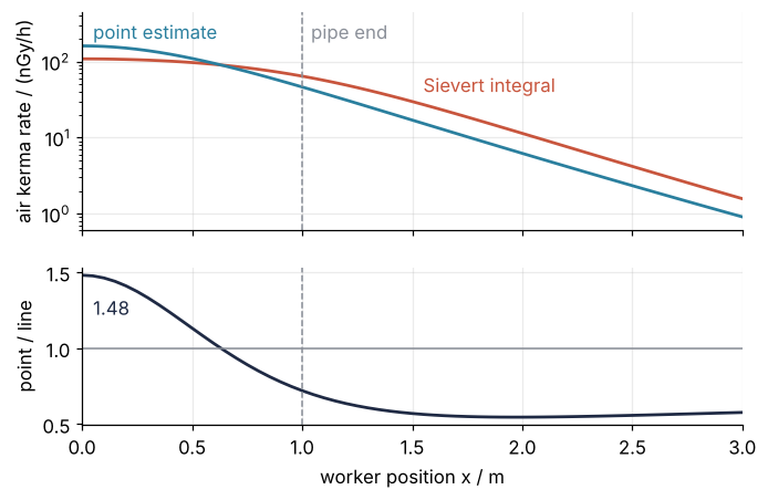
The ratio falls from 1.48 at the middle to 0.72 at the end of the pipe and 0.55 at 2 m, and is still 0.58 at 3 m. Once the worker leaves the middle, the part of the pipe in front of the worker is closer than its center and seen through less concrete, while the point estimate keeps everything at the center. From about 0.6 m on, that near part outweighs the far end, so the ratio crosses 1 before the pipe ends. From there on the point estimate is no longer conservative, the word shielding engineers use for an estimate that errs on the high side. It underestimates by almost a factor of two exactly where people walk around the end of a wall.

Pitfalls

Reading the uncollided dose as the dose. A survey meter behind the wall reads more than the 109 nGy/h. Behind more than a mean free path of concrete, photons that scattered once or several times and still reach the worker add a share comparable to the uncollided ones, and the Sievert integral counts none of them. The ratio of the total to the uncollided dose is the buildup factor, tabulated for a point isotropic source in an infinite medium in the ANSI/ANS-6.4.3 standard. Treat the result here as a lower bound and say so wherever you report it.

Mixing centimeters and meters. The tables give \(\mu\) in 1/cm. With \(t\) in meters, \(b\) comes out as 0.0138 instead of 1.38, the wall lets through 99 % instead of 25 %, and the dose is about four times too high without any error message. Keep one length unit throughout, centimeters here, and read the printed \(b\): a real shield is a few mean free paths thick, not a hundredth of one.

Unsigned angles past the end of the pipe. With the textbook \(F(\theta_1) + F(\theta_2)\) and both angles taken positive, a worker 1.5 m along the wall gets 101 nGy/h, nearly as much as in front of the middle, where Step 5 gives 30. That form assumes the foot of the perpendicular lies on the pipe. Use the signed angles and the difference of Step 3, which hold everywhere.

Variations

Another nuclide or shield. For caesium-137 behind steel, E holds the single line at 0.662 MeV with its yield of 0.851, and the table rows come from the iron entry of the same NIST table, around that energy, with a density of 7.874 g/cm³.
Scatter included. Multiply the integrand by a buildup factor \(B(b\sec u)\), evaluated along each slanted ray, from a fit such as the geometric-progression form whose coefficients come with ANSI/ANS-6.4.3. quad handles the new integrand unchanged.
Dose to a person. Multiply the air kerma at each energy by the conversion coefficient to ambient dose equivalent in ICRP Publication 74, the quantity a survey meter in sieverts displays.
A tank instead of a pipe. A disk or volume source adds a second coordinate to the integral; dblquad from the same module evaluates it.

Cheat sheet

mu = np.exp(np.interp(np.log(E), np.log(table_E), np.log(mu_rho))) * rho  # NIST rows, log-log
b = mu * t                                                    # mean free paths, t in cm
F = lambda th, b: quad(lambda u: np.exp(-b / np.cos(u)), 0, th)[0]  # Sievert integral
theta1, theta2 = np.arctan((-L/2 - x) / h), np.arctan((L/2 - x) / h)  # signed angles
phi = S_L * Y / (4 * np.pi * h) * (F(theta2, b) - F(theta1, b))  # uncollided fluence rate
K = np.sum(phi * E * muen_rho_air) * 1.602e-13 * 1e3          # air kerma rate, Gy/s