Bayesian model comparison with dynesty: one emission line or two?

The problem: one emission line or two?

A spectrometer with an instrumental line width of σ = 0.10 nm, measured on a calibration lamp, records an emission line a little too wide for one line and a little lopsided. Is it one line, or two closer together than the resolution? A fit cannot tell: two lines have four parameters against two and always fit at least as well. Here the two-line fit is better by 9.1 in ln L, and that settles nothing. Bayesian model comparison settles it, and dynesty computes the number it needs.

That number is the evidence, how probable the data are under a model before any parameter is fitted: the likelihood \(L(\theta)\) averaged over the prior \(\pi(\theta)\) of the parameters \(\theta\),

The ratio of two models' evidences, \(B = Z_2/Z_1\), is the Bayes factor. It pays the second model for a better fit and charges it for parameters the data did not need. dynesty computes \(\ln Z\) by nested sampling, with an error bar and posterior samples on the side.

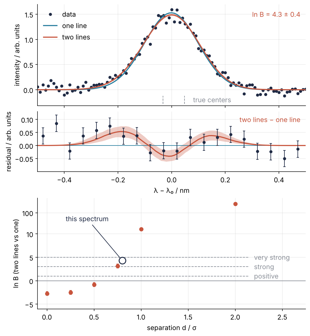
This is where we end up. Top: the spectrum with both models, where the evidence prefers two lines by odds of 76 to 1. Middle: what the second line buys, the excess on both flanks and the dip at the center that the one-line model leaves in the data. Bottom: the same comparison at six separations, two nested sampling runs of 250 live points each. Up to half a line width the data prefer one line; from one line width on the question is closed.

Setup

The spectrum is built from two lines whose amplitudes and centers we fix, which gives each result a truth to be held against. A single seeded noise draw serves every separation, so the sweep in Step 6 varies the separation and nothing else. For a measured spectrum, replace lam, y, and NOISE; no later cell needs editing.

import warnings
import numpy as np
import matplotlib.pyplot as plt
import dynesty

plt.rcParams.update({
    "figure.figsize": (7, 3.6), "figure.dpi": 110,
    "axes.spines.top": False, "axes.spines.right": False,
    "axes.grid": True, "grid.alpha": 0.25,
    "font.size": 11, "lines.linewidth": 1.8,
})
INK, ACCENT, SECOND, MUTED = "#1f2a44", "#c8553d", "#2a7f9e", "#8a8f98"

lam = np.linspace(-0.5, 0.5, 101)   # wavelength offset from the line, nm
SIGMA_LINE = 0.10                   # instrumental line width, nm, from the calibration lamp
NOISE = 0.07                        # noise per channel, in the intensity units of the spectrum
eps = np.random.default_rng(269).standard_normal(lam.size)

def line(lam, A, mu):
    return A * np.exp(-0.5 * ((lam - mu) / SIGMA_LINE) ** 2)

def spectrum(d):
    """Lines of 1.0 and 0.6 a separation d (nm) apart, placed so the centroid stays near 0."""
    return line(lam, 1.0, -0.4 * d) + line(lam, 0.6, 0.6 * d) + NOISE * eps

TRUTH = np.array([1.0, -0.032, 0.6, 0.048])   # A1, mu1, A2, mu2 of the main spectrum
y = spectrum(0.08)                            # separation 0.8 line widths
print(f"{lam.size} channels, peak / noise = {y.max() / NOISE:.0f}")

101 channels, peak / noise = 23

Step 1: Define the likelihood and the prior transform

The likelihood is the Gaussian one from MCMC with emcee, with its normalization constant kept. MCMC never needs the constant. The evidence contains it, and it cancels only in a difference of \(\ln Z\) between models of the same data.

The prior is where dynesty differs. Instead of a log-prior it takes a prior transform, a function that maps a point \(u\) of the unit cube to parameters so that uniform \(u\) gives draws from the prior. For independent priors, apply each prior's inverse cumulative distribution function to its own coordinate (Inverse transform sampling shows why). For a uniform prior that is lo + (hi - lo) * u; for a Gaussian one from an earlier measurement, mu0 + s0 * scipy.stats.norm.ppf(u), where ppf returns the value below which a fraction u of the standard normal lies. Here amplitudes are uniform in [0, 5] and centers in [-0.3, 0.3] nm, and the two-line transform sorts its centers so that line 1 is always the left one (Pitfall 1 says why it costs no evidence):

LN_NORM = lam.size * np.log(np.sqrt(2 * np.pi) * NOISE)

def log_gauss(y, model):
    return -0.5 * np.sum(((y - model) / NOISE) ** 2) - LN_NORM

def loglike_1(theta, y):
    A, mu = theta
    return log_gauss(y, line(lam, A, mu))

def loglike_2(theta, y):
    A1, mu1, A2, mu2 = theta
    return log_gauss(y, line(lam, A1, mu1) + line(lam, A2, mu2))

def prior_1(u, A_max=5.0):
    return np.array([A_max * u[0], -0.3 + 0.6 * u[1]])

def prior_2(u, A_max=5.0):
    mu1, mu2 = -0.3 + 0.6 * np.sort(u[[1, 3]])
    return np.array([A_max * u[0], mu1, A_max * u[2], mu2])

print("prior_2([0.5, 0.9, 0.5, 0.1]) =", prior_2(np.array([0.5, 0.9, 0.5, 0.1])))
print(f"ln L of the two-line model at the truth = {loglike_2(TRUTH, y):.1f}")
print(f"per channel, the constant adds {-LN_NORM / lam.size:.2f}")

prior_2([0.5, 0.9, 0.5, 0.1]) = [ 2.5  -0.24  2.5   0.24]
ln L of the two-line model at the truth = 121.1
per channel, the constant adds 1.74

The centers come back ordered, -0.24 and +0.24 nm from the coordinates 0.9 and 0.1. The transform does the job of emcee's log-prior and its walls: nothing outside the box can come out of it. The log-likelihood at the truth is positive, 121: with noise 0.07 the normalization alone adds 1.74 per channel, because the likelihood is a density in units of one over intensity.

Step 2: Run the nested sampler and read ln Z

Nested sampling turns the evidence into a one-dimensional integral. Call \(X(L^*)\) the prior mass where the likelihood exceeds a level \(L^*\): the fraction of prior draws that would fit at least that well. It runs from 1, for \(L^*\) below every point, to 0 at the maximum. Each slice \(dX\) of prior mass carries its likelihood \(L\), so \(Z = \int_0^1 L\,dX\), whatever the number of parameters.

dynesty measures \(X\) by counting. It draws 250 live points from the prior, discards the worst, makes its likelihood the new \(L^*\), and replaces it with a draw that has \(L > L^*\). The worst of 250 points sits on average at the bottom 1/250 of the remaining mass, so each replacement shrinks \(X\) by \(e^{-1/250}\), 0.4 %, and \(Z\) is summed over the discarded points, each \(L\) times the slice of \(X\) it took along. New draws come from a short random walk away from a live point that accepts only moves with \(L > L^*\) ("rwalk"; Pitfall 3 has the alternative). The run stops when the live points could add less than dlogz to \(\ln Z\), by default \(0.001\,(250-1) + 0.01 = 0.26\) here.

How far the run must go is set by the information \(H\), the number of factors of \(e\) by which the posterior is narrower than the prior. The posterior mass sits near \(\ln X \approx -H\), about \(250\,H\) iterations in:

sampler = dynesty.NestedSampler(loglike_1, prior_1, 2, logl_args=(y,), nlive=250,
                                sample="rwalk", rstate=np.random.default_rng(269))
sampler.run_nested(print_progress=False)
res_1 = sampler.results

H_1 = res_1.information[-1]
print(f"ln Z1 = {res_1.logz[-1]:.2f} ± {res_1.logzerr[-1]:.2f}")
print(f"H = {H_1:.1f}, 250 H = {250 * H_1:.0f}, iterations = {res_1.niter}, "
      f"likelihood calls = {sum(res_1.ncall)}")

ln Z1 = 105.22 ± 0.28
H = 8.9, 250 H = 2225, iterations = 2839, likelihood calls = 51766

\(\ln Z_1\) is positive for the reason Step 1 gave, and only differences of it mean anything. Its error, 0.28, shrinks as one over the square root of the number of live points: more live points buy precision, not a different answer. The 2,839 iterations are \(250\,H\) plus the stretch to the stop. Plot the share of \(Z\) per unit of \(\ln X\) to see where the evidence comes from:

Show code

Copy

weight = np.exp(res_1.logwt - res_1.logz[-1])        # each point's share of Z, summing to 1
density = weight / -np.gradient(res_1.logvol)        # share per unit of ln X
near_H = np.abs(res_1.logvol + H_1) < 2
fig, ax = plt.subplots(figsize=(7, 3.2))
ax.plot(res_1.logvol, density, color=ACCENT)
ax.fill_between(res_1.logvol, density, color=ACCENT, alpha=0.35, lw=0)
ax.axvline(-H_1, color=MUTED, ls="--", lw=1)
ax.text(-H_1 + 0.3, density.max() * 0.9, f"ln X = −H = −{H_1:.1f}", color=MUTED)
ax.set(xlabel="ln X (log of the prior mass above L*)", ylabel="share of Z per unit ln X",
       xlim=(res_1.logvol.min(), 0), ylim=(0, None))
plt.show()
print(f"peak at ln X = {res_1.logvol[np.argmax(density)]:.1f}; "
      f"share of Z within 2 of ln X = -H: {weight[near_H].sum():.0%}")

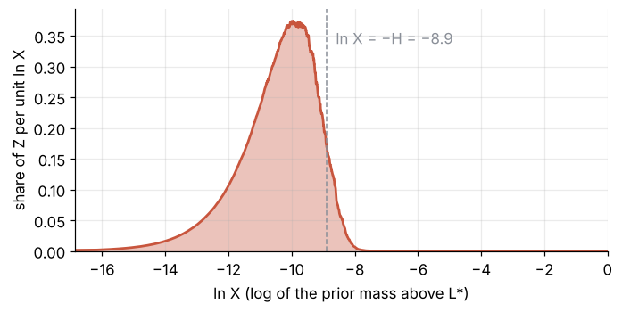
peak at ln X = -10.0; share of Z within 2 of ln X = -H: 70%

Seven tenths of the evidence come from four units of \(\ln X\) around \(-H\), where shrinking prior mass and growing likelihood balance. The best fit, at the far left, adds next to nothing: too little prior mass fits that well.

Step 3: Compare the two models with the Bayes factor

Wrap the call in a function, so that every later run is one line, and run the two-line model with four parameters. The two runs are independent, so their errors add in quadrature. The last discarded point is the one with the highest likelihood, so logl[-1] is the best fit:

def evidence(y, two=False, A_max=5.0, seed=269, prior=None, sample="rwalk"):
    """One nested sampling run of the one-line or two-line model; returns dynesty's results."""
    loglike, default_prior, ndim = (loglike_2, prior_2, 4) if two else (loglike_1, prior_1, 2)
    sampler = dynesty.NestedSampler(loglike, prior or default_prior, ndim,
                                    logl_args=(y,), ptform_args=(A_max,), nlive=250,
                                    sample=sample, rstate=np.random.default_rng(seed))
    sampler.run_nested(print_progress=False)
    return sampler.results

res_2 = evidence(y, two=True)
ln_B = res_2.logz[-1] - res_1.logz[-1]
ln_B_err = np.hypot(res_1.logzerr[-1], res_2.logzerr[-1])
d_lnL = res_2.logl[-1] - res_1.logl[-1]
print(f"ln Z2 = {res_2.logz[-1]:.2f} ± {res_2.logzerr[-1]:.2f}")
print(f"ln B  = {ln_B:.2f} ± {ln_B_err:.2f},  B = {np.exp(ln_B):.0f}")
print(f"best fit: ln L_max gains {d_lnL:.2f}, ln Z gains {ln_B:.2f}, Occam difference {d_lnL - ln_B:.2f}")

ln Z2 = 109.54 ± 0.32
ln B  = 4.33 ± 0.42,  B = 76
best fit: ln L_max gains 9.10, ln Z gains 4.33, Occam difference 4.78

Two lines are preferred by odds of 76 to 1. Kass and Raftery's scale for Bayes factors, which their 1995 paper states on \(2\ln B\), reads on ln B as positive above 1, strong above 3, and very strong above 5, so 4.33 is strong; Pitfall 2 says how far to trust such a reading. The best fit rose by 9.10 in ln L, but ln Z rose by only 4.33. The other 4.78 went to the two extra parameters. To a good approximation

with \(V_{\text{post}}\) and \(V_{\text{prior}}\) the volumes of posterior and prior. The second term is the log of the Occam factor, Step 2's shrink from prior to posterior, and it is always negative. For the two-line model it is 4.78 more negative than for the one-line model, because the data rule out most of the prior range of the two extra parameters.