Inverse transform sampling: from uniform random numbers to a star cluster (Python)

The question

A young star cluster of 10,000 solar masses is born with a spread of stellar masses that Edwin Salpeter measured in 1955 on stars near the Sun: the number of stars per unit mass falls as \(m^{-2.35}\), here from 0.1 to 100 solar masses. Stars heavier than about 8 solar masses end as supernovae. How many does the cluster have, and how would a simulation produce them one by one? The second half is what inverse transform sampling answers. The first half is a pair of integrals of the power law:

Show code

import numpy as np
import matplotlib.pyplot as plt
from scipy import stats

plt.rcParams.update({
    "figure.figsize": (7, 3.6), "figure.dpi": 110,
    "axes.spines.top": False, "axes.spines.right": False,
    "axes.grid": True, "grid.alpha": 0.25,
    "font.size": 11, "lines.linewidth": 1.8,
})
INK, ACCENT, SECOND, MUTED = "#1f2a44", "#c8553d", "#2a7f9e", "#8a8f98"

rng = np.random.default_rng(2026)
SLOPE = 2.35                       # dN/dm ∝ m^-SLOPE (Salpeter 1955)
M_LO, M_HI = 0.1, 100              # solar masses
M_CLUSTER = 1e4                    # solar masses
M_SN = 8                           # lightest star that ends as a supernova


def power_integral(p, a, b):
    """Integral of m^p from a to b, for p != -1."""
    return (b ** (p + 1) - a ** (p + 1)) / (p + 1)


A = M_CLUSTER / power_integral(1 - SLOPE, M_LO, M_HI)       # stars per unit mass at 1 solar mass
N_EXPECTED = A * power_integral(-SLOPE, M_LO, M_HI)
N_SN = A * power_integral(-SLOPE, M_SN, M_HI)
MASS_SN = A * power_integral(1 - SLOPE, M_SN, M_HI)
print(f"stars:              {N_EXPECTED:9,.1f}   mean mass {M_CLUSTER / N_EXPECTED:.3f} M☉")
print(f"above {M_SN} M☉:        {N_SN:9.2f}   {100 * N_SN / N_EXPECTED:.3f} % of the stars")
print(f"mass above {M_SN} M☉: {MASS_SN:9,.0f} M☉ {100 * MASS_SN / M_CLUSTER:.1f} % of the mass")

m = np.geomspace(M_LO, M_HI, 400)
per_decade = {"stars per decade of mass": A * np.log(10) * m ** (1 - SLOPE),
              "M☉ per decade of mass": A * np.log(10) * m ** (2 - SLOPE)}
shares = [f"{100 * N_SN / N_EXPECTED:.2f} % of stars", f"{100 * MASS_SN / M_CLUSTER:.0f} % of mass"]
fig, axes = plt.subplots(1, 2, figsize=(8, 3.4), layout="constrained")
heavy = m >= M_SN
for ax, (label, y), share in zip(axes, per_decade.items(), shares):
    ax.plot(m, y, color=INK)
    ax.fill_between(m[heavy], 0, y[heavy], color=ACCENT, alpha=0.35, lw=0)
    ax.text(0.97, 0.97, f"above {M_SN} M☉:\n{share}", transform=ax.transAxes, ha="right", va="top", color=ACCENT)
    ax.set(xscale="log", xlim=(M_LO, M_HI), ylim=(0, None), xlabel="mass / M☉", ylabel=label)
zoom = axes[0].inset_axes([0.5, 0.3, 0.47, 0.4])        # the tail of the count, magnified
tail = m >= 3
zoom.plot(m[tail], per_decade["stars per decade of mass"][tail], color=INK)
zoom.fill_between(m[heavy], 0, per_decade["stars per decade of mass"][heavy], color=ACCENT, alpha=0.35, lw=0)
zoom.set(xscale="log", xlim=(3, M_HI), ylim=(0, 1000), yticks=[0, 500, 1000], xticks=[10, 100])
zoom.set_xticks([], minor=True)
plt.show()

stars:               28,460.1   mean mass 0.351 M☉
above 8 M☉:            74.22   0.261 % of the stars
mass above 8 M☉:     1,390 M☉ 13.9 % of the mass

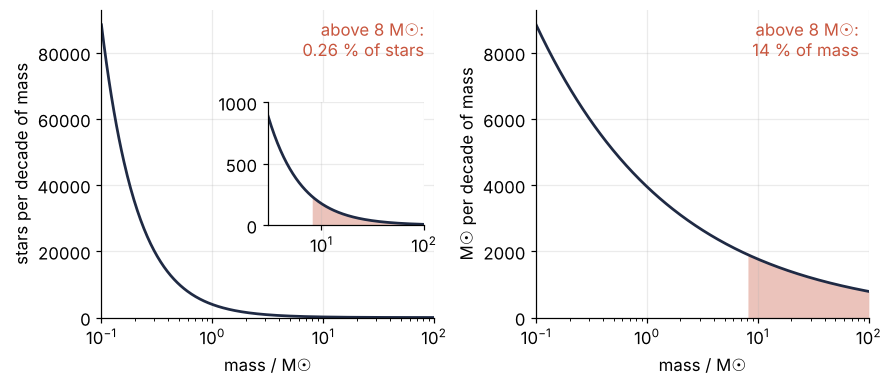
Stars per decade of mass (left) and mass per decade (right) against mass from 0.1 to 100 solar masses. Shaded above 8 solar masses: 0.26 % of the stars, visible only in the left inset, magnified 90 times, and 14 % of the mass.

The cluster has 28,460 stars with a mean mass of 0.351 solar masses. Only 74.2 of them, 0.26 %, are heavier than 8, and yet those few carry 13.9 % of the mass.

The curves count per decade of mass, the stars between \(m\) and \(10m\), instead of per solar mass. A decade is a factor of ten wide, so the count per decade is the density \(m^{-2.35}\) times \(m\) (and \(\ln 10\)), which falls as \(m^{-1.35}\); the mass per decade carries one more factor of \(m\) and falls as \(m^{-0.35}\). On the logarithmic axis every decade has the same width, so the shaded area is the share.

Two things are obvious from the curves. Light stars dominate the count, so completely that the stars above 8 show on the left only in the inset, magnified 90 times, while on the right the same few stars hold a share of the mass about 50 times their share of the count. Every number so far is an integral of the power law, and a pencil would have found it.

Less obvious: a simulation that follows each star, its pull on the others, its light, the moment it explodes, needs 28,460 individual masses, not an integral. NumPy's generator offers some thirty distributions, a Pareto law among them, but none that falls as \(m^{-2.35}\) between two cutoffs. How do uniform numbers become this list of masses, with the right 74 or so above 8?

The idea: uniform numbers falling onto a staircase

Start coarse, with five mass bins whose edges are at 0.1, 0.2, 0.5, 1, 8, and 100 solar masses. They hold 60.8 %, 27.8 %, 6.9 %, 4.2 %, and 0.26 % of the stars. Stacked from the lightest bin up, the shares form a staircase from 0 to 1, one riser per bin.

Now draw a uniform number u between 0 and 1, mark it on the vertical axis, and walk right until you hit a riser. That riser names the bin. Since u is uniform, the chance of hitting a riser is its height, the bin's share, so the bins come out in exactly the right proportions: 60.8 % of all u land on the first riser, and one in 383 on the last.

Make the bins finer and the staircase becomes a smooth curve, the cumulative distribution \(F(m)\), the share of stars lighter than \(m\). It is steep among the light stars and nearly flat above a few solar masses:

Show code

K = SLOPE - 1                                       # the exponent after integrating m^-SLOPE
SPAN = M_LO ** -K - M_HI ** -K


def cdf(m):
    return (M_LO ** -K - m ** -K) / SPAN


def salpeter_inverse(u):
    return (M_LO ** -K - u * SPAN) ** (-1 / K)


edges = np.array([0.1, 0.2, 0.5, 1, 8, 100])
centers = np.sqrt(edges[1:] * edges[:-1])          # each bin's stars placed at its middle on a log axis
steps = cdf(edges[1:])
u_mapped = [0.5, 0.9, 0.99]
print("bin shares / %:", "  ".join(f"{100 * s:.2f}" for s in np.diff(cdf(edges))))
for u in u_mapped:
    print(f"u = {u:4.2f}  ->  m = {salpeter_inverse(u):.3f} M☉")
print(f"F({M_SN} M☉) = {cdf(M_SN):.4f}")

fig, (ax1, ax2) = plt.subplots(2, 1, figsize=(7, 4.6), sharex=True, layout="constrained")
ax1.step(np.r_[M_LO, centers, M_HI], np.r_[0, steps, 1], where="post", color=INK)
for e in edges[1:-1]:
    ax1.axvline(e, color=MUTED, lw=1, ls="--")
for u in [0.30, 0.80, 0.97]:
    i = np.searchsorted(steps, u)
    ax1.annotate("", xy=(centers[i], 0), xytext=(centers[i], u),
                 arrowprops=dict(arrowstyle="->", color=ACCENT, lw=1.2))
    ax1.plot([M_LO, centers[i]], [u, u], color=ACCENT, lw=1.2)
ax1.annotate(f"last riser: {100 * (1 - steps[-2]):.2f} %", xy=(centers[-1], 0.99), xytext=(centers[-1], 0.55),
             ha="center", color=INK, arrowprops=dict(arrowstyle="->", color=INK, lw=1))
ax1.set(ylim=(0, 1.02), ylabel="cumulative share")
mm = np.geomspace(M_LO, M_HI, 400)
ax2.plot(mm, cdf(mm), color=INK)
zoom = ax2.inset_axes([0.68, 0.22, 0.3, 0.45])       # the top 1 % of u, magnified
zoom.plot(mm, cdf(mm), color=INK)
zoom.axhspan(cdf(M_SN), 1, color=ACCENT, alpha=0.35, lw=0)      # the stars above 8 M☉, shaded as in the first figure
zoom.axvline(M_SN, color=MUTED, lw=1, ls="--")
zoom.text(0.96, 0.08, f"top {100 * (1 - cdf(M_SN)):.2f} % of u:\nm > {M_SN} M☉", transform=zoom.transAxes,
          color=ACCENT, ha="right", va="bottom")
zoom.set(xscale="log", xlim=(3, M_HI), ylim=(0.99, 1), yticks=[0.99, 1], xticks=[10, 100])
zoom.set_xticks([], minor=True)
ax2.indicate_inset_zoom(zoom, edgecolor=MUTED, alpha=1, lw=1)
for u in u_mapped:
    m_u = salpeter_inverse(u)
    ax2.plot([M_LO, m_u, m_u], [u, u, 0], color=ACCENT, lw=1.2)
    ax2.text(m_u * 1.08, 0.04, f"{m_u:.3g}", color=ACCENT)
ax2.set(xscale="log", xlim=(M_LO, M_HI), ylim=(0, 1.02), xlabel="mass / M☉", ylabel="F(m)")
plt.show()

bin shares / %: 60.78  27.85  6.92  4.20  0.26
u = 0.50  ->  m = 0.167 M☉
u = 0.90  ->  m = 0.550 M☉
u = 0.99  ->  m = 3.011 M☉
F(8 M☉) = 0.9974

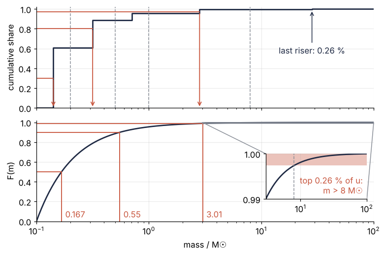
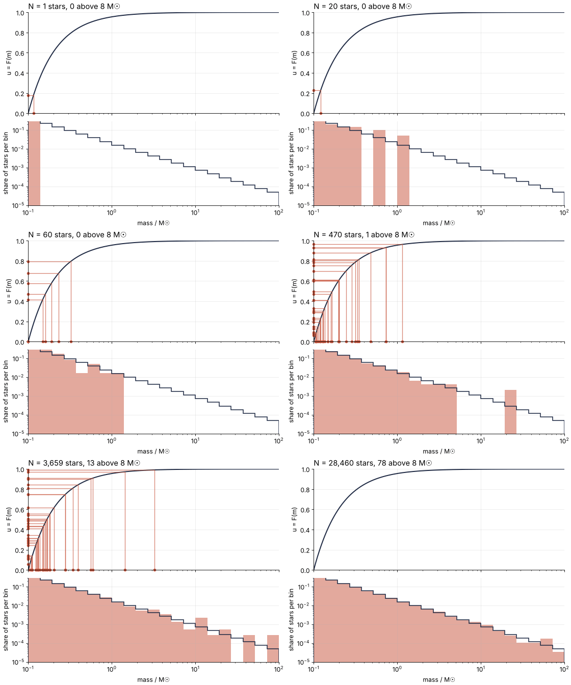
Top: five-bin staircase of cumulative shares against mass; three values of u run right to a riser and down to its bin. Bottom: the smooth F(m); u = 0.5, 0.9, 0.99 map to 0.167, 0.55, and 3.01 solar masses. The inset shows the top 1 % of u: its shaded top 0.26 % gives the stars above 8.

Half of all u fall below 0.5 and give stars lighter than 0.167 solar masses; u = 0.9 gives 0.55, and u = 0.99 gives 3.01. Every star above 8 comes from the top 0.26 % of the vertical axis, the shaded band in the inset, too thin to see at the scale of the panel. Here is the whole cluster arriving this way, in batches that grow from one star to a few thousand:

Top: uniform numbers u appear on the vertical axis, run right to the cumulative distribution of the Salpeter law, and drop to the mass axis. Bottom: the histogram of the masses drawn so far fills in toward the outline the power law predicts, with the counter reaching 28,460 stars and 78 above 8 solar masses.

Show code

"""CDF rain: uniform numbers u read backwards through the Salpeter CDF become stellar masses.

Renders ../../assets/cdf-rain.gif. Run it from any directory:

    python scene.py
"""
from pathlib import Path

import numpy as np
import matplotlib.pyplot as plt
from matplotlib.animation import FuncAnimation, PillowWriter
from PIL import Image, ImageSequence

OUT = Path(__file__).resolve().parents[2] / "assets" / "cdf-rain.gif"
INK, ACCENT, MUTED = "#1f2a44", "#c8553d", "#8a8f98"
plt.rcParams.update({"axes.spines.top": False, "axes.spines.right": False,
                     "axes.grid": True, "grid.alpha": 0.25, "font.size": 11})

# ---- the Salpeter law between 0.1 and 100 solar masses, and its inverse CDF
K, M_LO, M_HI = 1.35, 0.1, 100.0                         # K = 2.35 - 1
SPAN = M_LO**-K - M_HI**-K
cdf = lambda m: (M_LO**-K - m**-K) / SPAN
inverse = lambda u: (M_LO**-K - u * SPAN) ** (-1 / K)

# ---- the stars: 28,460 of them, released in batches that grow from 1 to about 2,000
N_STARS, N_FALL, N_HOLD = 28_460, 96, 14
rng = np.random.default_rng(2026)
u_all = rng.random(N_STARS)
m_all = inverse(u_all)
released = np.round(np.geomspace(1, N_STARS, N_FALL)).astype(int)
released = np.maximum.accumulate(np.maximum(released, np.arange(1, N_FALL + 1)))   # at least one new star per frame
released[-1] = N_STARS
frames = np.concatenate([released, np.full(N_HOLD, N_STARS)])                     # hold the last frame

edges = np.geomspace(M_LO, M_HI, 22)
expected = np.diff(cdf(edges))                                 # share of stars per bin, from the law
centers = np.sqrt(edges[1:] * edges[:-1])
m_curve = np.geomspace(M_LO, M_HI, 400)

# ---- figure, drawn once
fig, (ax1, ax2) = plt.subplots(2, 1, figsize=(7, 5.6), dpi=80, sharex=True,
                               height_ratios=[1.2, 1], layout="constrained")
ax1.plot(m_curve, cdf(m_curve), color=INK, lw=1.8)
rays = [ax1.plot([], [], color=ACCENT, lw=1.2, alpha=0.7)[0] for _ in range(30)]
(u_dots,) = ax1.plot([], [], "o", color=ACCENT, ms=4, clip_on=False)
(m_dots,) = ax1.plot([], [], "o", color=ACCENT, ms=4, clip_on=False)
for dots in (u_dots, m_dots):
    dots.set_in_layout(False)                                  # dots on the axes edges, not inside them
ax1.set(xscale="log", xlim=(M_LO, M_HI), ylim=(0, 1), ylabel="u = F(m)")
title = ax1.set_title("N = 0 stars", loc="left")

ax2.stairs(expected, edges, color=INK, lw=1.4, zorder=3)              # the law, drawn over the bars
bars = ax2.stairs(np.full_like(expected, 1e-6), edges, baseline=1e-6, fill=True, color=ACCENT, alpha=0.5, lw=0)
ax2.set(yscale="log", ylim=(1e-5, 0.3), xlabel="mass / M☉", ylabel="share of stars per bin")
fig.canvas.draw()
fig.set_layout_engine("none")                                  # lay out once, so the frames do not jitter


# ---- one frame: everything follows from the number of stars released so far
def update(n):
    i = np.searchsorted(released, n)
    start = released[i - 1] if i > 0 else 0
    new_u, new_m = u_all[start:n], m_all[start:n]
    for k, ray in enumerate(rays):                              # rays for at most 30 of the newest stars
        if k < new_u.size and n < N_STARS:
            ray.set_data([M_LO, new_m[k], new_m[k]], [new_u[k], new_u[k], 0])
        else:
            ray.set_data([], [])
    shown = slice(0, 0) if n == N_STARS else slice(0, 30)
    u_dots.set_data(np.full(new_u[shown].size, M_LO), new_u[shown])
    m_dots.set_data(new_m[shown], np.zeros(new_m[shown].size))
    counts, _ = np.histogram(m_all[:n], edges)
    bars.set_data(np.maximum(counts / n, 1e-6), edges)            # empty bins sit below the axis
    title.set_text(f"N = {n:,} stars, {np.sum(m_all[:n] > 8):,} above 8 M☉")


# ---- render, and read back what was written
OUT.parent.mkdir(exist_ok=True)
FuncAnimation(fig, update, frames=frames).save(OUT, writer=PillowWriter(fps=12))
plt.close(fig)
with Image.open(OUT) as im:
    seconds = sum(frame.info["duration"] for frame in ImageSequence.Iterator(im)) / 1000
    print(f"{OUT.name}: {im.width} x {im.height} px, {im.n_frames} frames, "
          f"{seconds:.1f} s, {OUT.stat().st_size / 1024:,.0f} kB")

The rule is to read the curve backwards: from u on the vertical axis to the mass on the horizontal one.

Turning the power law around

For the Salpeter law the curve can be read backwards with a formula. The share of stars lighter than \(m\) is the integral of \(m^{-2.35}\) from 0.1 up to \(m\), divided by the same integral up to 100. Integrating \(m^{-2.35}\) gives \(m^{-1.35}\) up to a constant, the exponent raised by one, so

\[F(m) = \frac{m_{\mathrm{lo}}^{-1.35} - m^{-1.35}}{m_{\mathrm{lo}}^{-1.35} - m_{\mathrm{hi}}^{-1.35}},\]

with \(m_{\mathrm{lo}} = 0.1\) and \(m_{\mathrm{hi}} = 100\) solar masses. Set \(F(m) = u\) and solve for \(m\):

\[m = \left[\, m_{\mathrm{lo}}^{-1.35} - u \left( m_{\mathrm{lo}}^{-1.35} - m_{\mathrm{hi}}^{-1.35} \right) \right]^{-1/1.35}.\]

That is the whole sampler. Draw 28,460 uniform numbers with rng.random from a generator seeded once (Random numbers with numpy.random covers the seeding), push them through the formula, and the result is a cluster:

Show code

N_STARS = round(N_EXPECTED)
u_cluster = rng.random(N_STARS)
masses = salpeter_inverse(u_cluster)
print(f"stars:        {N_STARS:,}")
print(f"total mass:   {masses.sum():,.0f} M☉")
print(f"above {M_SN} M☉:  {np.sum(masses > M_SN)}   expected {N_SN:.1f}")
print(f"below 1 M☉:   {np.mean(masses < 1):.4f}   expected {cdf(1):.4f}")

bins = np.geomspace(M_LO, M_HI, 31)
counts, _ = np.histogram(masses, bins)
width = np.diff(bins)
mid = np.sqrt(bins[1:] * bins[:-1])
full = counts > 0
fig, ax = plt.subplots()
ax.plot(mm, N_STARS * K * mm ** -SLOPE / SPAN, color=INK)
ax.errorbar(mid[full], counts[full] / width[full], yerr=np.sqrt(counts[full]) / width[full],
            fmt="o", ms=4, capsize=2, lw=1, color=ACCENT)
ax.axvline(M_SN, color=MUTED, lw=1, ls="--")
ax.text(M_SN * 1.15, 3e4, f"{np.sum(masses > M_SN)} stars\nabove {M_SN} M☉", color=ACCENT, va="top")
ax.set(xscale="log", yscale="log", xlim=(M_LO, M_HI), xlabel="mass / M☉",
       ylabel="stars per solar mass, dN/dm")
plt.show()

stars:        28,460
total mass:   10,080 M☉
above 8 M☉:  78   expected 74.2
below 1 M☉:   0.9552   expected 0.9554

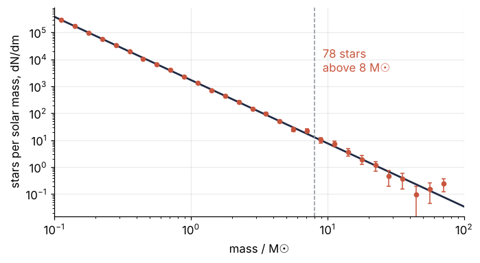
Stars per solar mass, dN/dm, of the 28,460 sampled masses on log-log axes from 0.1 to 100 solar masses, points with Poisson error bars on the straight m^-2.35 line. A dashed line at 8 solar masses; 78 sampled stars lie above it.

The y axis is each bin's count divided by its width in solar masses, which puts bins of different widths on the scale of the density, and the error bars are the square root of each count, the counting noise that Formalization takes up. The points follow the straight line of \(m^{-2.35}\) over three decades of mass. The sampled cluster has 78 stars above 8 solar masses where the integral expects 74.2, and 95.52 % of its stars are below 1 solar mass where the law says 95.54 %. Its total mass comes out at 10,080 solar masses, not 10,000, because a fixed number of stars carries a mass that scatters too.

When there is no formula: invert a table

Later work, collected by Pavel Kroupa in 2001, found fewer light stars than Salpeter's law predicts. In the version used here the slope is 1.3 below 0.5 solar masses and 2.3 above, over the same 0.1 to 100, the two pieces meeting at 0.5 without a jump. Two power laws could still be inverted by hand, but the table route works for any density you can evaluate, including a measured one:

Evaluate the density on 2,000 points over its range. A variable that spans decades, like these masses, gets points spaced evenly in its logarithm (np.geomspace); one that does not, a temperature or an angle, gets an even grid (np.linspace).
Integrate cumulatively with the trapezoid rule. On the logarithmic grid the steps are equal in \(\ln m\), so the rule runs over \(m f(m)\), since \(dm = m\, d(\ln m)\).
Normalize by the last value, so that the table of \(F\) runs from 0 to 1.
Invert by swapping the axes: with \(F\) as the x values, np.interp(u, F_table, x_table) on an even grid, np.exp(np.interp(u, F_table, np.log(m_table))) on the logarithmic one. np.interp needs its x values increasing, so where a gap in the density leaves \(F\) flat, drop the repeated values first.

Between the points of the table np.interp draws straight lines, so the accuracy depends on where the points sit. Spaced evenly in \(m\), the 2,000 points are 0.05 solar masses apart, and only 9 of them lie below 0.5, where \(F\) climbs from 0 to 0.73. Spaced evenly in \(\ln m\), each decade gets a third of them:

Show code

def kroupa(m):
    """Kroupa (2001) without its lowest piece: slopes 1.3 and 2.3, continuous at 0.5 M☉."""
    return np.where(m < 0.5, (m / 0.5) ** -1.3, (m / 0.5) ** -2.3)


def kroupa_cdf_exact(m):
    below = 0.5 ** 1.3 * power_integral(-1.3, M_LO, np.minimum(m, 0.5))
    above = 0.5 ** 2.3 * power_integral(-2.3, 0.5, np.maximum(m, 0.5))
    total = 0.5 ** 1.3 * power_integral(-1.3, M_LO, 0.5) + 0.5 ** 2.3 * power_integral(-2.3, 0.5, M_HI)
    return (below + above) / total


def cdf_table(m_grid):
    """Steps 1 to 3 on any grid, with the trapezoid rule in ln m."""
    g = m_grid * kroupa(m_grid)
    F = np.r_[0, np.cumsum(0.5 * (g[1:] + g[:-1]) * np.diff(np.log(m_grid)))]
    return F / F[-1]


u_test = np.random.default_rng(1).random(10**6)          # its own generator: the cluster's stream stays put
for name, m_grid in [("even in m   ", np.linspace(M_LO, M_HI, 2000)),
                     ("even in ln m", np.geomspace(M_LO, M_HI, 2000))]:
    F_table = cdf_table(m_grid)
    m_drawn = np.exp(np.interp(u_test, F_table, np.log(m_grid)))
    worst = np.max(np.abs(kroupa_cdf_exact(m_drawn) - u_test))
    print(f"grid {name}: {np.sum(m_grid < 0.5):4d} points below 0.5 M☉, worst |F(m) - u| = {worst:.1e}")

m_table = np.geomspace(M_LO, M_HI, 2000)
F_kroupa = cdf_table(m_table)
mass_per_star = (0.5 ** 1.3 * power_integral(-0.3, M_LO, 0.5) + 0.5 ** 2.3 * power_integral(-1.3, 0.5, M_HI))
stars_per_star = (0.5 ** 1.3 * power_integral(-1.3, M_LO, 0.5) + 0.5 ** 2.3 * power_integral(-2.3, 0.5, M_HI))
A_K = M_CLUSTER / mass_per_star
N_K = A_K * stars_per_star
N_K_SN = A_K * 0.5 ** 2.3 * power_integral(-2.3, M_SN, M_HI)
MASS_K_SN = A_K * 0.5 ** 2.3 * power_integral(-1.3, M_SN, M_HI)
print(f"Kroupa cluster of {M_CLUSTER:,.0f} M☉: {N_K:,.0f} stars, {N_K_SN:.1f} above {M_SN} M☉, "
      f"{100 * MASS_K_SN / M_CLUSTER:.0f} % of the mass")

fig, ax = plt.subplots(figsize=(7, 3.2))
ax.plot(mm, cdf(mm), color=INK)
ax.plot(m_table, F_kroupa, color=SECOND)
ax.text(0.13, 0.9, "Salpeter", color=INK)
ax.text(0.45, 0.35, "Kroupa, from the table", color=SECOND)
ax.set(xscale="log", xlim=(M_LO, M_HI), ylim=(0, 1.02), xlabel="mass / M☉", ylabel="F(m)")
plt.show()

grid even in m   :    9 points below 0.5 M☉, worst |F(m) - u| = 3.2e-03
grid even in ln m:  466 points below 0.5 M☉, worst |F(m) - u| = 1.1e-06
Kroupa cluster of 10,000 M☉: 15,681 stars, 111.3 above 8 M☉, 21 % of the mass

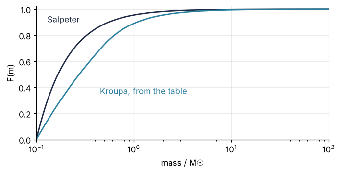
Cumulative distribution against mass on a log axis: the Kroupa law from a table in blue rises later than the Salpeter law in dark, because Kroupa has fewer light stars.

On the even grid the exact \(F\) of a drawn mass misses the u it came from, \(|F(m) - u|\), by up to 3.2e-3, worst where \(F\) is steep. On the logarithmic grid 466 points lie below 0.5 and the worst miss is 1.1e-6, on a million test values of u. The Kroupa cluster of 10,000 solar masses has 15,681 stars, of which 111.3 are expected above 8 solar masses, carrying 21 % of the mass. With fewer light stars, the same mass buys half again as many supernovae as Salpeter's 74.

Formalization

What the staircase showed holds for every continuous distribution. If \(F\) is the cumulative distribution of a random variable and \(U\) is uniform on \([0, 1)\), then

\[X = F^{-1}(U)\]

has the cumulative distribution \(F\). The proof is one line:

\[P\big(F^{-1}(U) \le m\big) = P\big(U \le F(m)\big) = F(m).\]

The first equality holds because \(F\) is increasing, so \(F^{-1}(U) \le m\) and \(U \le F(m)\) are the same event; the second because the chance that a uniform number lies below any value between 0 and 1 is that value. Where \(F\) is flat, over a gap that holds no probability, \(F^{-1}(u)\) is taken as \(\min\{m : F(m) \ge u\}\), the lightest mass that reaches u, and the gap never receives a sample.

With \(F\) in closed form the inversion is exact, and every difference between a sample and its law is counting noise. No formula for the density is required, only \(F\), from an integral or from a table.

The count above 8 is a Poisson count. Each star lands above 8 solar masses independently, with probability \(p = 0.00261\). When the chance per try is small and the tries are many, the number of hits scatters around its mean \(\lambda\) with a standard deviation of \(\sqrt{\lambda}\); that is the Poisson distribution, and \(\sqrt{\lambda}\) is called the Poisson error. Here \(\lambda = 74.2\) and \(\sqrt{\lambda} = 8.6\). Drawing 1,000 clusters with the same formula shows it:

Show code

n_above = np.array([np.sum(salpeter_inverse(rng.random(N_STARS)) > M_SN) for _ in range(1000)])
print(f"mean {n_above.mean():.1f}   standard deviation {n_above.std(ddof=1):.2f}")
print(f"Poisson: mean {N_SN:.1f}   standard deviation {np.sqrt(N_SN):.2f}")

k = np.arange(n_above.min(), n_above.max() + 1)
fig, ax = plt.subplots(figsize=(7, 3.2))
ax.hist(n_above, bins=np.arange(k[0] - 0.5, k[-1] + 1.5), color=ACCENT, alpha=0.6, lw=0)
ax.plot(k, 1000 * stats.poisson.pmf(k, N_SN), "o", ms=4, color=INK)
ax.axvline(np.sum(masses > M_SN), color=MUTED, lw=1, ls="--")
ax.set(xlabel=f"stars above {M_SN} M☉ in one cluster", ylabel="clusters of 1,000")
plt.show()

mean 74.6   standard deviation 8.55
Poisson: mean 74.2   standard deviation 8.61

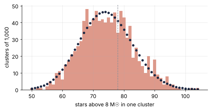
Histogram of the number of stars above 8 solar masses in 1,000 sampled clusters, centered near 74 with a spread of about 9, on top of Poisson probabilities for a mean of 74.2. A dashed line marks the 78 of the cluster above.

The 1,000 counts have a mean of 74.6 and a standard deviation of 8.55, against 74.2 and 8.61 from the Poisson formula. The dashed line is the seed-2026 cluster's 78, 0.4 Poisson errors above the expected 74.2: a typical draw, which is why I kept the seed.

A table is as good as its grid. Inverting a table adds the interpolation error of \(F\) to the sample, 1.1e-6 for the logarithmic grid of the Kroupa law. A share \(p\) estimated from \(N\) stars, each one in or out independently, scatters by the binomial standard error \(\sqrt{p(1-p)/N}\). For 28,460 stars that is 0.003 at most, for a share near one half, and 3.0e-4 for the 0.26 % above 8 solar masses: still about 270 times the table's error.

Where it stops. The method draws one variable at a time. A point uniform in a disk of radius \(R\) takes two steps: first the radius, whose cumulative distribution is the share of the disk's area inside \(r\), \(F(r) = r^2/R^2\), so \(r = R\sqrt{U}\); then the angle, uniform in \([0, 2\pi)\). Half the points lie inside \(R/\sqrt{2} = 0.71\,R\), not inside \(R/2\) as a uniform radius would have it. When the variables cannot be drawn one after another like this, rejection sampling or Markov chain Monte Carlo take over (MCMC with emcee, Hamiltonian Monte Carlo).

The simplest case of all is the exponential law of free paths, \(F(s) = 1 - e^{-\Sigma s}\) for a path length \(s\) in a medium with attenuation coefficient \(\Sigma\). It inverts to \(s = -\ln(1 - U)/\Sigma\), and since \(1 - U\) is as uniform as \(U\), particle transport codes write \(-\ln(U)/\Sigma\).

See it in code

SciPy has the truncated power law as scipy.stats.truncpareto. Its density is proportional to \(x^{-(b+1)}\) between scale and c * scale, so \(b = 1.35\), scale = 0.1 and c = 1000 is the Salpeter law between 0.1 and 100. Feed its ppf the same 28,460 uniform numbers as the hand-written inverse:

Show code

salpeter = stats.truncpareto(b=K, c=M_HI / M_LO, scale=M_LO)
m_scipy = salpeter.ppf(u_cluster)
print(f"largest relative difference from the formula: {np.max(np.abs(m_scipy / masses - 1)):.1e}")
print(f"expected above {M_SN} M☉:  N * sf(8) = {N_STARS * salpeter.sf(M_SN):.1f} ± {np.sqrt(N_STARS * salpeter.sf(M_SN)):.1f}")
print(f"drawn above {M_SN} M☉:     {np.sum(m_scipy > M_SN)}")

largest relative difference from the formula: 2.6e-13
expected above 8 M☉:  N * sf(8) = 74.2 ± 8.6
drawn above 8 M☉:     78

ppf, the percent point function, is SciPy's name for \(F^{-1}\); statisticians call it the quantile function. Every continuous distribution in scipy.stats has one, so dist.ppf(rng.random(n)) is inverse transform sampling for every distribution SciPy knows. Its partner sf, the survival function \(1 - F\), gives the expected count above 8. The library and the formula above agree to within 2.6e-13, which is rounding. The expected count is 74.2 ± 8.6, and the 78 drawn lie inside that by a wide margin.

Where it shows up

The star cluster is one case of a pattern that turns up wherever a simulation needs random numbers with a known law that the generator does not offer.

Particle transport (physics, engineering). A neutron or photon flies a free path drawn as \(-\ln(U)/\Sigma\), the exponential case of Formalization, and Monte Carlo transport builds a shield calculation on it. In neutron moderation the lethargy gain of a collision with hydrogen, the drop in the logarithm of the energy, is \(-\ln(U)\) by the same inversion.
Chemical kinetics and cell biology. In the Gillespie algorithm the waiting time to the next reaction is exponential with the total rate \(a_0\), so inversion gives \(\tau = -\ln(U)/a_0\). The Gillespie algorithm draws it with rng.exponential, which produces the same law by a faster route.
Seismology (geology). The Gutenberg-Richter law says the number of earthquakes of magnitude at least \(M\) falls as \(10^{-bM}\) with \(b\) near 1. Inverting it gives \(M = M_{\min} - \log_{10}(U)/b\), one line for the magnitudes of a synthetic earthquake catalog.
Grain sizes (geology, engineering). Crushed rock and powders often follow the Rosin-Rammler distribution, \(F(d) = 1 - \exp(-(d/d_{63})^n)\) with \(d_{63}\) the sieve size that 63 % of the material passes, the Weibull law under another name. It inverts to \(d = d_{63}(-\ln U)^{1/n}\), so a simulated sieve test needs one line.
Photon energies (physics). The Planck spectrum has no cumulative distribution in elementary functions. Radiative-transfer codes tabulate it once and interpolate, the table route of the Kroupa law.

Each case needs the integral of its density once, by hand or as a table, and after that every random number costs one evaluation of \(F^{-1}\).

The question

The idea: uniform numbers falling onto a staircase

Turning the power law around

When there is no formula: invert a table

Formalization

See it in code

Where it shows up

Further reading