MCMC with emcee: the half-life and background of a counting experiment

The problem: how long does the isotope live, and what is background?

A detector counts a short-lived isotope for 60 one-minute intervals. In the first minute it registers 41 counts, in each of the last ten minutes between 2 and 5, and about 3 of those per minute are background that would be there without the source. The expected count in minute \(i\) is

\[\mu_i = A\,2^{-t_i/T_{1/2}} + B ,\]

with \(t_i\) the middle of the interval, \(A\) the initial rate, \(T_{1/2}\) the half-life, and \(B\) the background. The two you want are the half-life and the background.

Markov chain Monte Carlo (MCMC) with emcee takes the Poisson statistics as they are. The usual move, least squares with \(\sqrt{N}\) error bars, does not: at 4 counts per minute it treats a 2 as a precise number and a 6 as a loose one, although both scatter around 4 by the same amount. Instead of one best point, MCMC returns thousands of parameter sets drawn from the posterior: how probable each combination of \(A\), \(T_{1/2}\), and \(B\) is, given the counts.

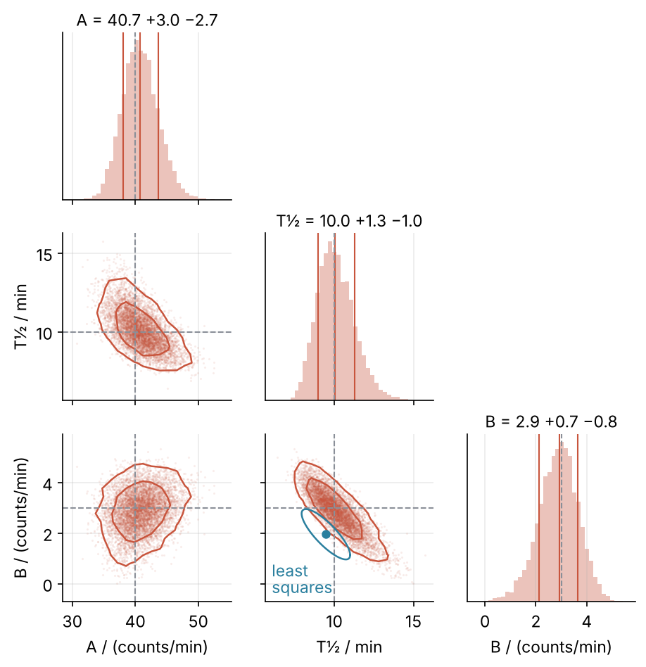
Corner plot of the posterior of A, half-life, and background. The half-life against background cloud tilts down (r = -0.84) and stretches toward long half-lives; the least-squares ellipse has the same tilt but sits below the true background.

This is where we end up. The half-life against background cloud tilts down: a longer half-life comes with less background, and the two have to be reported together, each with a credible interval, the range that holds 68 % of the posterior probability. The picture is 32 walkers run for 5,000 steps, with the start of the run thrown away.

Setup

The counts are simulated from known values, \(A = 40\) per minute, \(T_{1/2} = 10\) min, and \(B = 3\) per minute, so that every answer below can be checked. The generator is NumPy's seeded default_rng (Random numbers with numpy.random explains it). Swap in your own t and N and the rest runs unchanged.

import numpy as np
import matplotlib.pyplot as plt
import emcee
from scipy.optimize import curve_fit

plt.rcParams.update({
    "figure.figsize": (7, 3.6), "figure.dpi": 110,
    "axes.spines.top": False, "axes.spines.right": False,
    "axes.grid": True, "grid.alpha": 0.25,
    "font.size": 11, "lines.linewidth": 1.8,
})
INK, ACCENT, SECOND, MUTED = "#1f2a44", "#c8553d", "#2a7f9e", "#8a8f98"

A_true, T_half_true, B_true = 40.0, 10.0, 3.0   # counts/min, min, counts/min

def rate(t, A, T_half, B):
    return A * 2.0 ** (-t / T_half) + B

rng = np.random.default_rng(93)
t = np.arange(60) + 0.5                          # interval midpoints / min
N = rng.poisson(rate(t, A_true, T_half_true, B_true))

print("first ten:", N[:10])
print("last ten: ", N[-10:])

first ten: [41 42 42 27 27 41 23 24 24 27]
last ten:  [4 5 4 2 3 4 4 4 4 5]

Step 1: Write the log-posterior as a Python function

Three terms carry the rest of the tutorial. The likelihood is the probability of the observed counts for a given set of parameters. The prior is what you believe about the parameters before you see any counts. The posterior is a probability distribution over the parameters given the counts, and by Bayes' theorem it is proportional to likelihood times prior.

emcee asks for one function: the logarithm of likelihood times prior, up to a constant. For Poisson counts with expected values \(\mu_i\) the log-likelihood is

\[\ln L = \sum_i \left( N_i \ln \mu_i - \mu_i \right),\]

with \(\ln N_i!\) dropped because it does not depend on the parameters. The prior is flat inside physical walls and -np.inf outside, and it is checked first, so that a negative rate never reaches the logarithm:

def log_prior(theta):
    A, T_half, B = theta
    if 0 < A < 1000 and 0 < T_half < 100 and 0 < B < 100:
        return 0.0
    return -np.inf

def log_prob(theta):
    lp = log_prior(theta)
    if not np.isfinite(lp):
        return -np.inf
    mu = rate(t, *theta)
    return lp + np.sum(N * np.log(mu) - mu)

def log_like_gauss(theta, x, y, sigma, model):   # for data with Gaussian error bars; not used here
    return -0.5 * np.sum(((y - model(x, *theta)) / sigma)**2)

for label, theta in [("truth", (40, 10, 3)), ("T½ = 30 min", (40, 30, 3)), ("B = -1/min", (40, 10, -1))]:
    print(f"{label:12s} log_prob = {log_prob(np.array(theta, float)):8.1f}")

truth        log_prob =   1373.6
T½ = 30 min  log_prob =   1085.8
B = -1/min   log_prob =     -inf

The 1373.6 at the truth means nothing on its own, because of the dropped constant. Differences mean everything: the 30-minute half-life is 287.7 lower, so it is \(e^{288}\) times less probable: excluded.

If your data are measurements with Gaussian error bars \(\sigma_i\), the log-likelihood is \(-\chi^2/2\) instead, the log_like_gauss above, and its maximum is the least-squares fit (Least squares: what a fit minimizes explains \(\chi^2\)). To sample your own problem, write the log-likelihood of how your data scatter, add the log-prior, and nothing else below changes. The Poisson sum is used here because at 4 counts per minute the Gaussian approximation fails, as Step 5 shows.

Step 2: Start the walkers and run the sampler

A walker is one point in the three-dimensional parameter space. emcee moves an ensemble of them together: each walker proposes a jump along the line through itself and another walker, the stretch move of Goodman and Weare. The jump lands at the other walker plus \(z\) times the separation, with \(z\) drawn between 1/2 and 2. It is taken with a probability equal to the smaller of 1 and \(z^{d-1}\) times the ratio of the new to the old posterior value, with \(d = 3\) the number of parameters. The factor \(z^{d-1}\) is the Jacobian of stretching along the line in \(d\) dimensions; without it the walkers would sample a distorted distribution. So walkers spend time in each region in proportion to its posterior probability, and the positions they visit are draws from the posterior. The ratio is the exponential of a difference of log-probabilities, which is why the constant dropped in Step 1 never matters. Each step depends only on the current positions, which is the "Markov chain" in MCMC.

emcee refuses to run with fewer than twice as many walkers as parameters; 32 for three is comfortable. They start in a small ball of 1 % scatter, because the stretch move needs walkers at different points to have lines to move along. The center is read off the data, with the half-life deliberately at 15 min:

B_guess = N[-10:].mean()
guess = np.array([N[0] - B_guess, 15.0, B_guess])
nwalkers, ndim = 32, 3
p0 = guess * (1 + 0.01 * rng.standard_normal((nwalkers, ndim)))

sampler = emcee.EnsembleSampler(nwalkers, ndim, log_prob)
sampler.random_state = np.random.RandomState(93).get_state()   # the sampler ignores rng (Pitfalls)
sampler.run_mcmc(p0, 5000)

print("chain shape:", sampler.get_chain().shape)
print(f"mean acceptance fraction: {sampler.acceptance_fraction.mean():.2f}")

chain shape: (5000, 32, 3)
mean acceptance fraction: 0.64

That is 160,000 parameter sets in a few seconds. The acceptance fraction is the share of proposed jumps taken under the rule above, here about two in three.

Step 3: Check convergence with traces and the autocorrelation time

How long a walker needs to forget where it was is the autocorrelation time \(\tau\), which emcee estimates per parameter, and it sets how much of the chain to use. I discard the first 5 \(\tau\), to drop the start before the walkers reach the posterior, and keep every \(\tau/2\)-th step, because rows closer than that are near copies of each other:

tau = sampler.get_autocorr_time()                 # raises below 50 tau, the tol of emcee.autocorr.integrated_time
discard = int(5 * tau.max())
thin = int(tau.max() / 2)
n_eff = nwalkers * (5000 - discard) / tau.max()   # one independent sample per tau steps and walker

print("tau / steps:", np.round(tau, 1))
print(f"discard = {discard}, thin = {thin}, independent samples ≈ {n_eff:.0f}")

tau / steps: [45.9 37.8 37.7]
discard = 229, thin = 22, independent samples ≈ 3329

\(\tau\) also says whether the run was long enough. A chain shorter than 50 \(\tau\) holds too few independent stretches for emcee to trust its estimate of \(\tau\), and get_autocorr_time raises an error. Here 5,000 steps is over 100 \(\tau\). Plot every walker's position against the step number for the first 1,000 steps, one panel per parameter, with a gray line at discard:

Show code

chain = sampler.get_chain()
labels = ["A / (counts/min)", "T½ / min", "B / (counts/min)"]
truths = [A_true, T_half_true, B_true]

fig, axes = plt.subplots(3, 1, figsize=(7, 6.6), sharex=True)
for k, ax in enumerate(axes):
    ax.plot(chain[:1000, :, k], color=INK, alpha=0.15, lw=0.6)
    ax.axhline(truths[k], color="white", lw=3, zorder=3)            # a gap so that the truth shows on the walkers
    ax.axhline(truths[k], color=MUTED, ls="--", lw=1.2, zorder=4)
    ax.axvline(discard, color=MUTED, lw=1)
    ax.set(ylabel=labels[k])
axes[0].text(discard, 1.02, "discard", color=MUTED, ha="center", va="bottom",   # above the panel, clear of the walkers
             transform=axes[0].get_xaxis_transform())
axes[-1].set(xlabel="step", xlim=(0, 1000))
plt.show()

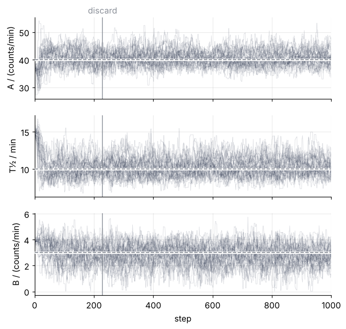
Traces of the 32 walkers for A, half-life, and background against step number, first 1,000 steps. The walkers leave the deliberately wrong 15-minute start within about 50 steps and then wander in one band around the dashed true values. A vertical line at step 229 marks the discarded start.

The walkers leave the 15-minute start within about 50 steps and then wander in one band around the truth. That first stretch is burn-in, and the 229 steps left of the line are generous against it. Keeping every 22nd step saves memory and time and loses almost nothing. It does not make the kept rows independent: rows 22 steps apart are half a \(\tau\) apart and still correlated.

What sets the precision of every percentile in Step 4 is the 3,329 independent samples, not the 160,000 sets or the rows you keep (The standard error of the mean shows why).

Step 4: Read off the half-life and background with credible intervals

get_chain with flat=True stacks the kept steps of all walkers into one array, one row per sample. Every question about the parameters is now a question about these rows. The 16th and 84th percentiles enclose the middle 68 %, the share a Gaussian puts within ±1σ, so the interval reads like a lab error bar without assuming a Gaussian:

flat = sampler.get_chain(discard=discard, thin=thin, flat=True)
lo, med, hi = np.percentile(flat, [16, 50, 84], axis=0)
r = np.corrcoef(flat.T)

print("rows:", flat.shape)
for name, unit, k in [("A", "counts/min", 0), ("T½", "min", 1), ("B", "counts/min", 2)]:
    print(f"{name:2s} = {med[k]:5.2f} +{hi[k] - med[k]:.2f} / -{med[k] - lo[k]:.2f} {unit}")
print(f"r(T½, B) = {r[1, 2]:.2f}")

rows: (6912, 3)
A  = 40.70 +2.97 / -2.67 counts/min
T½ = 10.02 +1.26 / -1.04 min
B  =  2.91 +0.74 / -0.79 counts/min
r(T½, B) = -0.84

The truth sits inside each interval. The half-life interval is lopsided, longer on the upper side, because a long half-life is easier to hide under background than a short one; a ± cannot say that. The correlation of -0.84 means the two errors are not independent: a half-life at the top of its interval goes with a background at the bottom of its own. Report them together, with \(r\).

Each row is also a curve. Draw 200 rows and take percentiles of rate(t, *row) at every time:

Show code

rows = flat[rng.choice(len(flat), 200, replace=False)]
curves = np.array([rate(t, *row) for row in rows])
c_lo, c_med, c_hi = np.percentile(curves, [16, 50, 84], axis=0)
width = c_hi - c_lo
print(f"band width: {width[0]:.1f} counts/min at the start ({100 * width[0] / c_med[0]:.0f} %), "
      f"{width[-1]:.1f} at the end ({100 * width[-1] / c_med[-1]:.0f} %)")

fig, ax = plt.subplots()
ax.plot(t, N, "o", color=INK, ms=4)
ax.plot(t, c_med, color=ACCENT)
ax.fill_between(t, c_lo, c_hi, color=ACCENT, alpha=0.30, lw=0)
ax.axhline(B_true, color=MUTED, ls="--", lw=1)
ax.text(1, B_true + 1.2, "true background B", color=MUTED)
ax.set(xlabel="t / min", ylabel="counts per minute", xlim=(0, 60), ylim=(-1, None))   # a zero count stays whole
plt.show()

band width: 5.6 counts/min at the start (13 %), 1.0 at the end (28 %)

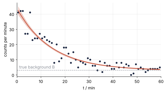
Counts per minute against time over 60 minutes, falling from about 40 to about 4. Line: posterior median model. Band: 68 % of posterior curves, widest in absolute terms at the start and, relative to the counts, at late times, where the decay tail meets the dashed true background of 3 per minute.

The dots have no error bars on purpose: \(\sqrt{N}\) bars are the picture this tutorial argues against. In absolute terms the band is widest at the start, where everything hangs on \(A\). Relative to the counts it is twice as wide at the end, 28 % against 13 %, where tail and background are hard to tell apart.

Step 5: Compare with a least-squares fit

The fit most people would do is curve_fit with \(\sqrt{N}\) error bars (curve_fit from the ground up covers the call). It maximizes the Gaussian likelihood of Step 1 with \(\sigma_i = \sqrt{N_i}\), so this is one likelihood against another, not MCMC against fitting:

sigma = np.sqrt(np.maximum(N, 1))   # a zero count would get a zero error bar
popt, pcov = curve_fit(rate, t, N, p0=guess, sigma=sigma, absolute_sigma=True)
perr = np.sqrt(np.diag(pcov))

print(f"T½ = {popt[1]:.2f} ± {perr[1]:.2f} min")
print(f"B  = {popt[2]:.2f} ± {perr[2]:.2f} counts/min")
print(f"r(T½, B) = {pcov[1, 2] / (perr[1] * perr[2]):.2f}")

T½ = 9.47 ± 1.02 min
B  = 1.95 ± 0.66 counts/min
r(T½, B) = -0.82

pcov is the covariance matrix of the fitted parameters. The square roots of its diagonal, perr, are the ± errors, and \(r\) is the off-diagonal element divided by both errors. absolute_sigma=True takes the \(\sqrt{N}\) bars as true standard deviations, not rescaled to the scatter. The correlation agrees with the posterior. The background does not: 1.95 is 1.6 standard errors below the true 3. Bad luck on this data set, or the method? Fit 300 simulated experiments:

B_fits = []
for _ in range(300):
    N_sim = rng.poisson(rate(t, A_true, T_half_true, B_true))
    p, _ = curve_fit(rate, t, N_sim, p0=guess, sigma=np.sqrt(np.maximum(N_sim, 1)), absolute_sigma=True)
    B_fits.append(p[2])

print(f"mean fitted B over 300 experiments: {np.mean(B_fits):.2f} counts/min (truth {B_true:.1f})")

mean fitted B over 300 experiments: 1.84 counts/min (truth 3.0)

It is the method. A count that fluctuates down gets a smaller error bar and pulls the curve harder, and at 4 counts per minute those fluctuations are a large share of the signal. The Poisson likelihood has no such weights. Fit counts with the Poisson likelihood.

Step 6: Draw the corner plot of the joint posterior

The corner plot puts each parameter's histogram on the diagonal and each pair's samples below it, with contours that enclose 68 % and 95 % of the samples. The helper levels finds the histogram height above which those shares lie. On the half-life and background panel the least-squares result joins in, as a point and its 68 % ellipse:

def levels(H, shares=(0.95, 0.68)):
    h = np.sort(H.ravel())[::-1]
    cum = np.cumsum(h) / h.sum()
    return [h[np.searchsorted(cum, s)] for s in shares]

names = ["A", "T½", "B"]
edges = np.percentile(flat, [0.05, 99.95], axis=0).T               # shared axis limits per parameter
lims = [(a - 0.2 * (b - a), b + 0.2 * (b - a)) for a, b in edges]

fig, axes = plt.subplots(3, 3, figsize=(7, 7))
for i in range(3):
    for j in range(3):
        ax = axes[i, j]
        if j > i:
            ax.set_visible(False)
            continue
        if i == j:
            ax.hist(flat[:, i], bins=40, range=lims[i], color=ACCENT, alpha=0.35, lw=0)
            for q in (lo[i], med[i], hi[i]):
                ax.axvline(q, color=ACCENT, lw=1)
            ax.set_yticks([])
            ax.text(0.5, 1.04, f"{names[i]} = {med[i]:.1f} +{hi[i] - med[i]:.1f} −{med[i] - lo[i]:.1f}",
                    transform=ax.transAxes, ha="center")
        else:
            H, xe, ye = np.histogram2d(flat[:, j], flat[:, i], bins=20, range=[lims[j], lims[i]])
            ax.plot(flat[:, j], flat[:, i], ".", color=ACCENT, ms=1, alpha=0.1)
            ax.contour((xe[1:] + xe[:-1]) / 2, (ye[1:] + ye[:-1]) / 2, H.T,
                       levels=levels(H), colors=ACCENT, linewidths=1.2)
            ax.axhline(truths[i], color=MUTED, ls="--", lw=1)
            ax.set_ylim(lims[i])
        ax.axvline(truths[j], color=MUTED, ls="--", lw=1)
        ax.set_xlim(lims[j])
        ax.locator_params(nbins=4)                  # the same ticks for a parameter in row and column
        if i == 2:
            ax.set_xlabel(labels[j])
        else:
            ax.set_xticklabels([])
        if j == 0 and i > 0:
            ax.set_ylabel(labels[i])
        elif i != j:
            ax.set_yticklabels([])

# least squares on the T½-B panel: the Cholesky factor of the 2 x 2 covariance
# maps a unit circle, scaled to the 68 % radius of two parameters, onto the ellipse
ax = axes[2, 1]
L = np.linalg.cholesky(pcov[1:, 1:])
phi = np.linspace(0, 2 * np.pi, 200)
ellipse = popt[1:, None] + np.sqrt(-2 * np.log(1 - 0.68)) * L @ np.array([np.cos(phi), np.sin(phi)])
ax.plot(*ellipse, color=SECOND, lw=1.2)
ax.plot(popt[1], popt[2], "o", color=SECOND, ms=5)
ax.text(0.04, 0.05, "least\nsquares", color=SECOND, linespacing=1.0, transform=ax.transAxes)
fig.align_labels()
plt.show()

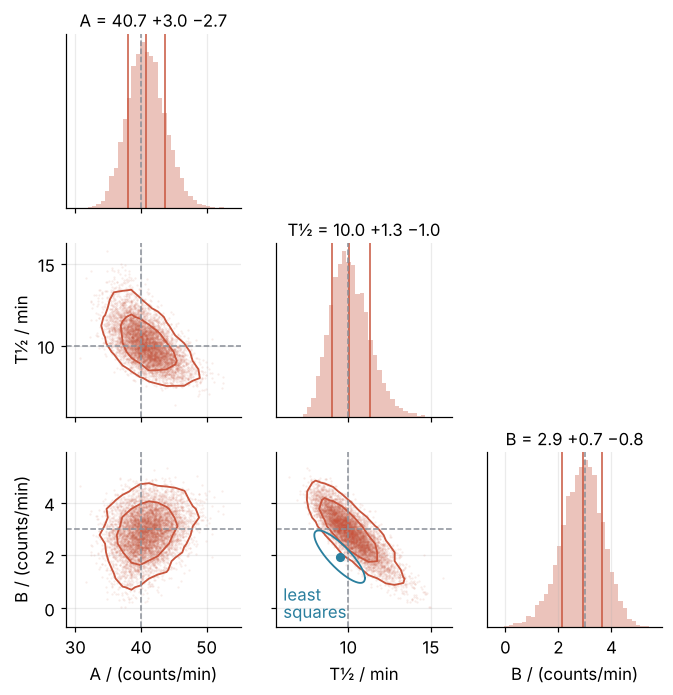
Corner plot of the posterior of A, half-life, and background. The half-life against background cloud tilts down (r = -0.84) and stretches toward long half-lives; the least-squares ellipse has the same tilt but sits below the true background.

The three lines in each diagonal histogram are the 16th, 50th, and 84th percentiles, printed above it. The half-life and background cloud tilts down with r = -0.84 and stretches toward long half-lives, the skew Step 4 printed as +1.3 / -1.0. The least-squares ellipse has the same tilt and a symmetric shape, and it sits below the dashed truth in \(B\).

Pitfalls

A parameter the data do not pin down. A flat prior that never ends is called improper, because its total probability is infinite, and it is harmless only as long as the data pin the parameter down. Lose the first 30 minutes (the detector was switched on late) and drop the upper wall on \(A\):

import logging
logging.getLogger("emcee").setLevel(logging.ERROR)   # its warnings say what the printed tau says

late = t > 30
def log_prob_open(theta):
    A, T_half, B = theta
    if not (A > 0 and 0 < T_half < 100 and 0 < B < 100):
        return -np.inf
    mu = rate(t[late], *theta)
    return np.sum(N[late] * np.log(mu) - mu)

open_sampler = emcee.EnsembleSampler(nwalkers, ndim, log_prob_open)
open_sampler.random_state = np.random.RandomState(93).get_state()
open_sampler.run_mcmc(p0, 5000)
open_chain = open_sampler.get_chain()
for n in (1000, 2500, 5000):
    A_med, T_med, _ = np.median(open_chain[n - 1], axis=0)
    tau_n = emcee.autocorr.integrated_time(open_chain[:n], quiet=True)
    print(f"step {n}: median A = {A_med:9.2e} /min, median T½ = {T_med:5.2f} min, tau(T½) = {tau_n[1]:4.0f}")

step 1000: median A =  9.24e+03 /min, median T½ =  2.54 min, tau(T½) =  105
step 2500: median A =  2.80e+20 /min, median T½ =  0.28 min, tau(T½) =  281
step 5000: median A =  2.87e+53 /min, median T½ =  0.12 min, tau(T½) =  502

By step 5,000 the median rate is \(3 \times 10^{53}\) per minute and the median half-life 7 s, because a huge rate decaying fast fits the tail as well as a moderate one. The symptom is medians that drift with every thousand steps and a \(\tau\) in the hundreds that keeps growing. The late data do not constrain \(A\), and no prior can repair that: a wall on \(A\) would only move the pile-up to the wall, and the half-life would then be the prior answering. So use a proper prior and check that the posterior does not pile up against any wall. If it does, the parameter is not measured, and the cure is data that see the decay. The main data set passes: its posterior sits far from every wall, with only a thin tail toward \(B = 0\).

Chains that have not mixed. Run 300 steps and ask for \(\tau\):

short = emcee.EnsembleSampler(nwalkers, ndim, log_prob)
short.random_state = np.random.RandomState(93).get_state()
short.run_mcmc(p0, 300)
try:
    short.get_autocorr_time()
except emcee.autocorr.AutocorrError as err:
    print("AutocorrError:", str(err).splitlines()[0])
print("tau with quiet=True:", np.round(short.get_autocorr_time(quiet=True), 1))

try:
    short.run_mcmc(np.tile(guess, (nwalkers, 1)), 10)   # every walker at the same point
except ValueError as err:
    print("ValueError:", err)

AutocorrError: The chain is shorter than 50 times the integrated autocorrelation time for 3 parameter(s). Use this estimate with caution and run a longer chain!
tau with quiet=True: [18.7 18.9 22.5]
ValueError: Initial state has a large condition number. Make sure that your walkers are linearly independent for the best performance

That is the check from Step 3 doing its job. With quiet=True it returns a \(\tau\) of about 19 to 23 steps, half the value of the long run, so a short chain looks better mixed than it is. Start every walker at the same point and emcee refuses with the ValueError, for the reason given in Step 2. The fix is a chain longer than 50 \(\tau\), started from distinct points.

The seed that does not reach the sampler. EnsembleSampler keeps its own legacy RandomState, copied from NumPy's global state when the sampler is created. The default_rng(93) of the setup does not touch it, and emcee.State(p0, random_state=93) with an integer is silently ignored. The symptom is digits that change on every run. The fix is the line from Step 2, sampler.random_state = np.random.RandomState(93).get_state(), on every sampler you create.

Variations

A measured background. A separate background run of known length gives \(B\) with an error. Replace the flat prior on \(B\) by a Gaussian or a Gamma log-prior (the Gamma is a distribution for positive quantities only).
Two isotopes. Two decay terms make five parameters. Require \(T_{1/2,1} < T_{1/2,2}\) in the prior, so that the walkers cannot swap the labels.
A derived quantity. The decay constant \(\ln 2 / T_{1/2}\) or the counts expected in the first hour: transform the rows of flat and take percentiles again, no new run.
Long runs. emcee.backends.HDFBackend writes the chain to disk as it runs, so that a run can be resumed or inspected. It needs h5py.

Cheat sheet

def log_prob(theta):                                                  # log(likelihood x prior) + const
    if not np.all((lower < theta) & (theta < upper)): return -np.inf  # flat prior inside walls
    return np.sum(N * np.log(model(t, *theta)) - model(t, *theta))    # Gaussian: -0.5 * np.sum(((y - model(x, *theta)) / sigma)**2)
sampler = emcee.EnsembleSampler(nwalkers, ndim, log_prob)             # nwalkers >= 2 * ndim
sampler.random_state = np.random.RandomState(seed).get_state()        # the only seed it obeys
p0 = guess * (1 + 0.01 * rng.standard_normal((nwalkers, ndim)))       # a small ball, not one point
sampler.run_mcmc(p0, nsteps)
tau = sampler.get_autocorr_time()                                     # raises if nsteps < 50 tau
flat = sampler.get_chain(discard=int(5 * tau.max()), thin=int(tau.max() / 2), flat=True)
lo, med, hi = np.percentile(flat, [16, 50, 84], axis=0)               # np.corrcoef(flat.T) for r