findiff.PDE with mixed boundary conditions: seepage under a dam

The problem: how much water passes under a dam, and how hard does it push?

A concrete dam with a flat base 20 m wide sits on 20 m of sand over impermeable bedrock. The reservoir stands 8 m above the tailwater, and water seeps through the sand under the dam. The engineer wants the uplift, how hard that water pushes up on the base, and the seepage, how much of it passes per day. Both come from a PDE with mixed boundary conditions, which findiff turns into one sparse linear system.

The unknown is the hydraulic head h, the height to which water would rise in a standpipe, measured from the ground surface. The tailwater stands level with the ground, so h = 0 there. Water flows down the head gradient at a rate proportional to it (Darcy's law), and what flows into a piece of soil flows out again, so \(\nabla^2 h = 0\). The head is fixed on the ground upstream (h = 8 m) and downstream (h = 0). No water crosses the base of the dam, the bedrock, or the two far sides: \(\partial h/\partial n = 0\) there. The type of condition changes twice along the top edge, which is where hand-built stencils go wrong.

For sand of unlimited depth, Harr's classical solution gives the head under the base, \(h = (H/\pi)\arccos(2x/B)\), with \(H\) the 8 m, \(B\) the width of the base, and \(x\) measured from its center. It checks the uplift, not the seepage, which on deep sand has no finite value.

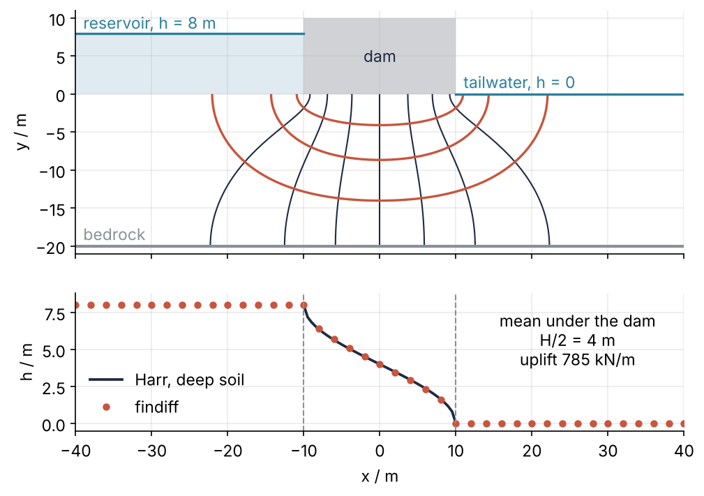
Top: the soil under a 20 m dam, with lines of equal head 1 m apart and three flow lines running from the reservoir under the dam to the tailwater. Bottom: head along the ground surface in m; the findiff dots lie on Harr's curve under the dam.

This is where we end up: the flow net, lines of equal head in dark blue and flow lines in red, over the head along the ground against Harr's curve. Per meter of dam, the uplift is 785 kN and the seepage 3.7 m³ a day. Step 6 draws it.

Setup

findiff installs with pip install findiff.

import numpy as np
import matplotlib.pyplot as plt
from findiff import Diff, PDE, BoundaryConditions
from scipy.integrate import trapezoid, cumulative_trapezoid
from scipy.special import ellipk

H = 8.0          # m, reservoir level above the tailwater
B = 20.0         # m, width of the dam's base
T = 20.0         # m, depth of the sand layer
W = 120.0        # m, width of the section we model
d = 0.5          # m, grid spacing
k = 1e-5         # m/s, hydraulic conductivity of a fine silty sand
gamma_w = 9.81   # kN/m^3, unit weight of water

plt.rcParams.update({                      # the look of every figure below
    "figure.figsize": (7.5, 4.6), "figure.dpi": 110,
    "axes.spines.top": False, "axes.spines.right": False,
    "axes.grid": True, "grid.alpha": 0.25,
    "font.size": 11, "lines.linewidth": 1.8,
})
INK, ACCENT, SECOND, MUTED = "#1f2a44", "#c8553d", "#2a7f9e", "#8a8f98"

print(f"dam {B:.0f} m wide, head drop {H:.0f} m, sand {T:.0f} m deep, grid spacing {d} m")

dam 20 m wide, head drop 8 m, sand 20 m deep, grid spacing 0.5 m

Step 1: Lay out the grid and the Laplacian

The soil becomes a grid of nodes 0.5 m apart, from the bedrock at y = −20 m to the ground at y = 0, and 120 m wide so the side walls sit far from the dam. With indexing="ij", axis 0 is x and axis 1 is y, so Diff(0, d) is \(\partial/\partial x\) at spacing d and the Laplacian a sum of two squares:

x = np.arange(-W / 2, W / 2 + d / 2, d)
y = np.arange(-T, d / 2, d)                 # y = 0 is the ground surface, up is +y
X, Y = np.meshgrid(x, y, indexing="ij")     # axis 0 is x, axis 1 is y
shape = X.shape

L = Diff(0, d)**2 + Diff(1, d)**2
print(f"grid {shape[0]} x {shape[1]} nodes")
print(f"largest |L(x² - y²)| = {np.abs(L(X**2 - Y**2)).max():.1e}")

grid 241 x 41 nodes
largest |L(x² - y²)| = 1.5e-11

The Laplacian of \(x^2 - y^2\) is zero, and findiff returns at most 1.5e-11 on every node, edges included: rounding. At an edge a centered stencil would need a node outside the grid, so findiff uses a one-sided one. Both are exact on a quadratic.

A steady problem has no time steps. It is one linear equation per node, and L.matrix shows them:

A = L.matrix(shape)
print(f"{A.shape[0]:,} x {A.shape[1]:,} sparse matrix, {A.nnz:,} nonzeros")

9,881 x 9,881 sparse matrix, 49,691 nonzeros

Row n says "the Laplacian at node n equals the right-hand side at node n". findiff numbers the nodes as NumPy flattens the grid, so node (i, j) is row 41i + j (41 nodes along y). That makes 9,881 unknowns, and a typical row holds five nonzeros, the node and its four neighbors.

Step 2: Describe each edge with BoundaryConditions

On the edges those rows are the wrong equations: a bedrock node is one where no water crosses. Each assignment to a BoundaryConditions object replaces the rows of the nodes it indexes. A Dirichlet row becomes "h here equals this value", a Neumann row "this derivative here equals this value". The matrix stays square, and when two assignments touch a node, the last one is its row.

A Dirichlet condition takes a number or an array. A Neumann condition takes a tuple (Diff(axis, d), value), and the value is the derivative along the positive axis, \(\partial h/\partial x\) or \(\partial h/\partial y\). That is not the convention of py-pde, whose derivative is taken along the outward normal, so on the bedrock the two differ in sign. A value may be a full-grid array, from which findiff picks the entries of the nodes it sets. So the edges become a function of three arrays, which Step 3 first feeds a known solution:

def edges(x, d, g, gx, gy):
    """Fixed head g on the ground outside the dam; dh/dx = gx and dh/dy = gy on every other edge."""
    under_dam = np.abs(x) < B / 2           # strictly inside: heel and toe keep the fixed head
    bc = BoundaryConditions(np.shape(g))
    bc[0, :] = (Diff(0, d), gx)             # upstream side wall
    bc[-1, :] = (Diff(0, d), gx)            # downstream side wall
    bc[:, 0] = (Diff(1, d), gy)             # bedrock
    bc[under_dam, -1] = (Diff(1, d), gy)    # base of the dam
    bc[~under_dam, -1] = g                  # ground surface, assigned last
    return bc

For the dam, g is 8 m upstream and 0 downstream, and both derivatives are zero. The fixed head comes last, so the two top corners and the heel and toe, the two ends of the base, carry it, as in Harr's solution. The new rows sit in the sparse matrix bc.lhs. Count the nonzeros in those of the ground surface, rows 41i + 40:

bc = edges(x, d, np.where(X < 0, H, 0.0), 0, 0)
n = np.arange(shape[0]) * shape[1] + shape[1] - 1           # node (i, -1) is row 41i + 40
fixed = np.count_nonzero(bc.lhs[n].toarray(), axis=1) == 1   # a Dirichlet row holds a single 1
print(f"fixed head at {fixed.sum()} nodes, no flow at {(~fixed).sum()}")
print(f"no flow from x = {x[~fixed].min():.1f} m to {x[~fixed].max():.1f} m")

fixed head at 202 nodes, no flow at 39
no flow from x = -9.5 m to 9.5 m

The 39 no-flow nodes lie strictly under the base, and the heel and toe at ±10 m are fixed with the other 200.

Step 3: Solve, check on a known function, and read the uplift

First solve a problem whose answer you know, with the same mixed layout. Take \(g = x^2 - y^2\), give the edges its value and its derivatives \(\partial g/\partial x = 2x\) and \(\partial g/\partial y = -2y\), and the solver should return \(g\). PDE(L, f, bc) takes the operator, the right-hand side f on every node, and the conditions:

g = X**2 - Y**2
h_check = PDE(L, np.zeros(shape), edges(x, d, g, 2 * X, -2 * Y)).solve()
print(f"largest error {np.abs(h_check - g).max():.1e} m")

largest error 1.0e-10 m

The stencils are exact on a quadratic, so an error could only come from the conditions or the solve, and 1e-10 m is rounding. The check carries over to any problem: pick a smooth function g, set the edges from it and f to L(g), here zero, and compare. It does not test the stencil. Refinement and a wider domain do (Step 4 and the pitfalls).

Now the dam, one sparse solve:

h = PDE(L, np.zeros(shape), edges(x, d, np.where(X < 0, H, 0.0), 0, 0)).solve()

base = np.abs(x) <= B / 2                   # heel and toe included
x_base, h_base = x[base], h[base, -1]
harr = H / np.pi * np.arccos(2 * x_base / B)
uplift = gamma_w * trapezoid(h_base, x_base)
i0 = np.argmin(np.abs(x))                   # the node under the center of the dam
print(f"head at the base center  {h[i0, -1]:.3f} m")
print(f"uplift                   {uplift:.1f} kN/m   (gamma_w H/2 B = {gamma_w * H / 2 * B:.1f})")
print(f"largest gap from Harr    {np.abs(h_base - harr).max():.2f} m")

head at the base center  4.000 m
uplift                   784.8 kN/m   (gamma_w H/2 B = 784.8)
largest gap from Harr    0.06 m

Head becomes pressure through \(p = \gamma_w (h - y)\). The base lies at y = 0, so the pressure there is \(\gamma_w h\) and the uplift its integral across the base. Had the tailwater stood t meters deep, you would put y = 0 at its surface, the base at y = −t, and the uplift would grow by \(\gamma_w t B\) while not a drop more water flowed: only differences in head drive it. The mean head under the base is exactly H/2, because swapping upstream and downstream maps the problem onto itself with h turned into H − h.

Step 4: Integrate the flux for the seepage rate

Darcy's law gives the volume of water that crosses a square meter of a vertical section per second, \(v_x = -k\,\partial h/\partial x\), called the Darcy flux. It is not the speed of the water: the water squeezes through the pores, a third of the section in sand, and moves about three times faster. Diff(0, d) applied to the solution gives the derivative. Integrate \(v_x\) over the vertical section under the center of the dam:

dhdx = Diff(0, d)(h)
q = trapezoid(-k * dhdx[i0, :], y)          # m^3/s per meter of dam
print(f"q = {q:.3g} m³/s per m = {q * 86400:.2f} m³/day per meter of dam")

q = 4.27e-05 m³/s per m = 3.69 m³/day per meter of dam

One section catches all of it. No water leaves through the bedrock or the base, and what enters upstream leaves downstream, so every vertical section under the dam carries the same q. To check the number on finer grids, wrap the solve in a function:

def solve_dam(T, W=120.0, d=0.5):
    x = np.arange(-W / 2, W / 2 + d / 2, d)
    y = np.arange(-T, d / 2, d)
    X, Y = np.meshgrid(x, y, indexing="ij")
    h = PDE(Diff(0, d)**2 + Diff(1, d)**2, np.zeros(X.shape),
            edges(x, d, np.where(X < 0, H, 0.0), 0, 0)).solve()
    return x, y, h

def seepage(x, y, h):
    dhdx = Diff(0, x[1] - x[0])(h)
    return trapezoid(-k * dhdx[np.argmin(np.abs(x)), :], y)

runs = {dd: solve_dam(T, d=dd) for dd in [1.0, 0.5, 0.25]}
print("q / (m³/day per m):  " + "   ".join(f"d = {dd} m: {seepage(*run) * 86400:.4f}" for dd, run in runs.items()))

q / (m³/day per m):  d = 1.0 m: 3.6945   d = 0.5 m: 3.6895   d = 0.25 m: 3.6869

The answer moves by 0.2 % between 1 m and 0.25 m spacing, so 3.69 m³/day per meter of dam is converged. The head field does not contain k, so the seepage scales with k and the head does not: sand ten times more permeable loses ten times the water and pushes up on the dam exactly as hard.

Step 5: Make the layer deeper

Harr's solution is for sand without a bottom. Rerun at four depths and compare the head under the base with his curve, the uplift, where it acts, and the seepage. The last column is the closed form from conformal mapping for a flat base of width B on a layer of depth T, \(q/(kH) = K(1-m)/\big(2K(m)\big)\) with \(m = \tanh^2\big(\pi B/(4T)\big)\). \(K\) is the complete elliptic integral of the first kind, scipy.special.ellipk, which takes the parameter \(m\), not the modulus.

print(" T/m   gap from Harr/m   uplift/(kN/m)   resultant/m   q/(kH)   closed form")
for depth in [5.0, 10.0, 20.0, 40.0]:
    xs, ys, hs = solve_dam(depth)
    on_base = np.abs(xs) <= B / 2
    xb, hb = xs[on_base], hs[on_base, -1]
    gap = np.abs(hb - H / np.pi * np.arccos(2 * xb / B)).max()
    shift = -trapezoid(hb * xb, xb) / trapezoid(hb, xb)     # upstream of the center
    m = np.tanh(np.pi * B / (4 * depth))**2
    print(f"{depth:4.0f}   {gap:15.2f}   {gamma_w * trapezoid(hb, xb):13.1f}   {shift:11.2f}"
          f"   {seepage(xs, ys, hs) / (k * H):6.3f}   {ellipk(1 - m) / (2 * ellipk(m)):11.3f}")

 T/m   gap from Harr/m   uplift/(kN/m)   resultant/m   q/(kH)   closed form
   5              0.37           784.8          2.87    0.205         0.205
  10              0.17           784.8          2.69    0.348         0.347
  20              0.06           784.8          2.58    0.534         0.533
  40              0.02           784.8          2.53    0.731         0.743

The uplift is 784.8 kN/m at every depth, by Step 3's symmetry. Depth changes the shape. In a shallow layer the head under the base falls more nearly in a straight line, which moves the resultant toward the heel, 2.87 m upstream of the center at 5 m depth, against Harr's B/8 = 2.50 m. Its lever arm about the toe, the point the dam would tip over, is then 12.87 m instead of 12.50 m, about 3 % more overturning moment. The seepage grows with every meter of sand and matches the closed form to one unit in the third decimal down to 20 m. At 40 m it falls 1.6 % short, and the third pitfall says why.

Step 6: Draw the flow net

Water does not cross a flow line, so the flow between the bedrock and a point is the same all along a flow line. That flow is the stream function \(\psi\), and integrating \(v_x\) upward from the bedrock gives it:

psi = cumulative_trapezoid(-k * dhdx, y, axis=1, initial=0)   # flow between bedrock and node
print(f"psi under the base center {psi[i0, -1] * 86400:.2f} m³/day per m, the same as q")

psi under the base center 3.69 m³/day per m, the same as q

The bedrock is the flow line \(\psi = 0\), the base of the dam the flow line \(\psi = q\), and two lines a value \(\Delta\psi\) apart carry \(\Delta\psi\) between them. Contour \(h\) in steps of H/8, \(N_d = 8\) head drops, and \(\psi\) in steps of q/4, \(N_f = 4\) flow channels. With square cells each channel carries \(kH/N_d\), so engineers drawing this by hand read off \(q \approx kH\,N_f/N_d = 0.5\,kH\), against findiff's 0.534 kH.

fig, (ax, ax2) = plt.subplots(2, 1, sharex=True, figsize=(7.5, 5.4),
                              gridspec_kw={"height_ratios": [3.0, 1.6]})
ax.contour(X, Y, h, levels=np.arange(1, H), colors=INK, linewidths=1.0)
ax.contour(X, Y, psi, levels=q * np.array([0.25, 0.5, 0.75]), colors=ACCENT, linewidths=1.6)
ax.fill_between([-B / 2, B / 2], 0, 10, color=MUTED, alpha=0.4, lw=0)
ax.text(0, 5, "dam", ha="center", va="center", color=INK)
ax.fill_between([-40, -B / 2], 0, H, color=SECOND, alpha=0.15, lw=0)
ax.plot([-40, -B / 2], [H, H], color=SECOND, lw=1.6)
ax.text(-39, H + 0.6, "reservoir, h = 8 m", color=SECOND)
ax.plot([B / 2, 40], [0, 0], color=SECOND, lw=1.6)
ax.text(B / 2 + 1, 0.8, "tailwater, h = 0", color=SECOND)
ax.axhline(-T, color=MUTED, lw=2)
ax.text(-39, -T + 0.8, "bedrock", color=MUTED)
ax.set(ylabel="y / m", xlim=(-40, 40), ylim=(-T - 1, 11))
ax.set_aspect("equal", adjustable="box", anchor="S")     # one meter is one meter: the flow net's cells stay square

ax2.plot(x_base, harr, color=INK, label="Harr, deep soil")
ax2.plot(x[::4], h[::4, -1], "o", color=ACCENT, ms=4, label="findiff")
for edge in [-B / 2, B / 2]:
    ax2.axvline(edge, color=MUTED, lw=1, ls="--")
ax2.text(26, 7.6, "mean under the dam\nH/2 = 4 m\nuplift 785 kN/m", ha="center", va="top")
ax2.set(xlabel="x / m", ylabel="h / m", ylim=(-0.5, 8.8))
ax2.legend(frameon=False, loc="lower left")
plt.show()

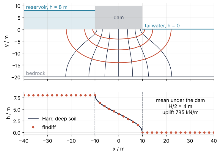
Top: the soil under a 20 m dam, x and y in m, with lines of equal head 1 m apart and three flow lines from the reservoir under the dam to the tailwater; both crowd at the heel and the toe. Bottom: head on the ground surface in m; the findiff dots lie on Harr's curve under the dam, mean 4 m.

The equipotentials and the flow lines crowd at the heel and the toe, where the fixed head meets the no-flow base. Under the dam the dots sit on Harr's curve to 0.06 m.

Pitfalls

The derivative along the wrong axis, or with the wrong sign. A slip of one character, Diff(0, d) for the nodes under the base:

import warnings

bc = edges(x, d, np.where(X < 0, H, 0.0), 0, 0)
bc[np.abs(x) < B / 2, -1] = (Diff(0, d), 0)        # should be Diff(1, d)
with warnings.catch_warnings(record=True) as caught:
    warnings.simplefilter("always")
    h_wrong = PDE(L, np.zeros(shape), bc).solve()
print(f"{caught[0].category.__name__}: {caught[0].message}; every node NaN: {np.isnan(h_wrong).all()}")

MatrixRankWarning: Matrix is exactly singular; every node NaN: True

In the row picture of Step 2, those rows now involve only nodes on the top edge: "no change along x" from a fixed 8 m at the heel to a fixed 0 at the toe, which no head satisfies. A wrong sign is worse, because it runs. Write the bedrock's value the py-pde way, as the outward derivative \(2y\) instead of \(\partial g/\partial y = -2y\), and the check of Step 3 is off by thousands of meters:

h_sign = PDE(L, np.zeros(shape), edges(x, d, g, 2 * X, 2 * Y)).solve()
print(f"largest error {np.abs(h_sign - g).max():.1e} m")

largest error 1.9e+03 m

Run that check every time you change a condition.

Gradients at the corners. Where the fixed head meets the no-flow base, the head gradient grows without bound, and refining the grid only shows more of it. The exit gradient, the head drop per meter where water rises out of the ground past the toe, is the number that decides piping: sand carried away by the outflow until a pipe erodes back under the dam, which starts as the gradient nears a critical value of about 1. Read it at a stated distance from the toe:

for dd, (xs, ys, hs) in runs.items():
    grad = np.hypot(Diff(0, dd)(hs), Diff(1, dd)(hs))[:, -1]
    exit_1m = -Diff(1, dd)(hs)[np.argmin(np.abs(xs - (B / 2 + 1))), -1]
    print(f"d = {dd:4} m   largest gradient on the surface {grad.max():.2f}   1 m past the toe {exit_1m:.2f}")
print(f"Harr, deep soil, 1 m past the toe: {H / (np.pi * np.sqrt((B / 2 + 1)**2 - (B / 2)**2)):.2f}")

d =  1.0 m   largest gradient on the surface 1.00   1 m past the toe 0.50
d =  0.5 m   largest gradient on the surface 1.41   1 m past the toe 0.52
d = 0.25 m   largest gradient on the surface 2.00   1 m past the toe 0.52
Harr, deep soil, 1 m past the toe: 0.56

The node maximum doubles from 1 m to 0.25 m spacing and will keep growing. One meter past the toe the gradient has settled, a little under Harr's deep-soil value. Report gradients at a distance from the corner, never the largest node value.

A domain too narrow. The side walls are no-flow edges that the real ground does not have, and they squeeze the flow. In a 40 m layer:

for width in [60.0, 120.0, 240.0]:
    print(f"W = {width:5.0f} m   q = {seepage(*solve_dam(40.0, W=width)) * 86400:.2f} m³/day per m")

W =    60 m   q = 4.31 m³/day per m
W =   120 m   q = 5.06 m³/day per m
W =   240 m   q = 5.14 m³/day per m

Sixty meters of width loses 16 % of the seepage, and the 120 m of Step 5 still loses 1.6 % against 240 m, close to its shortfall against the closed form in Step 5. Put the side walls two or three layer depths from the dam and check by doubling W.

Variations

Anisotropic soil. Layered sediments conduct better along the bedding than across it. Use kx * Diff(0, d)**2 + ky * Diff(1, d)**2 as the operator, and \(k_x\) in the flux.
A leaky clay blanket. A bottom that lets some water through takes a Robin condition, \(\alpha h + \beta\,\partial h/\partial y = g\), written as the four-tuple (alpha, Diff(1, d), beta, g). findiff's docstring calls this one the mixed condition; here mixed meant two types on one edge.
A relief well or recharge. A source or sink in the soil is a nonzero right-hand side in place of np.zeros(shape).
The same problem elsewhere. A strip electrode on an insulating surface, or a strip heater on an insulated plate, is the same mixed problem with the potential or the temperature in place of the head.

Cheat sheet

X, Y = np.meshgrid(x, y, indexing="ij")          # axis 0 is x, axis 1 is y
L = Diff(0, dx)**2 + Diff(1, dy)**2               # L(u) applies it; L.matrix(shape) is the system
bc = BoundaryConditions(X.shape)                  # each assignment replaces the rows of its nodes
bc[0, :] = 1.0                                    # Dirichlet: a number or a full-grid array
bc[:, 0] = (Diff(1, dy), g)                       # Neumann: du/dy along +y, not the outward normal
bc[:, -1] = (alpha, Diff(1, dy), beta, g)         # Robin: alpha u + beta du/dy = g
u = PDE(L, f, bc).solve()                         # the last assignment at a node wins
# check: edges from a known g, f = L(g), compare u with g
q = trapezoid(-k * Diff(0, dx)(u)[i, :], y)       # flux through the section x = x[i]