Surface temperature of an airless planet: day, night, and below the ground (Python)

The problem: a day and a night on the Moon's equator

A day on the Moon lasts 29.53 Earth days from noon to noon, and there is no atmosphere to keep the surface warm through the two weeks of night. Balance the absorbed sunlight against thermal radiation and the surface temperature on the equator comes out at 386 K at noon and absolute zero all night. The Diviner radiometer on the Lunar Reconnaissance Orbiter measures about 95 K just before dawn. The difference is heat conduction into the regolith, the loose rock and dust on top: the ground stores heat by day and gives it back at night.

The temperature \(T\) below the surface follows the heat equation, with the depth \(z\) pointing down, \(\rho\) the density, \(c\) the specific heat, and \(k\) the conductivity:

\[ \rho c\,\frac{\partial T}{\partial t} = k\,\frac{\partial^2 T}{\partial z^2} . \]

At the top, whatever the surface absorbs and does not radiate is conducted down:

\[ -k\,\frac{\partial T}{\partial z}\Big|_{z=0} = (1 - A)\,S\,\max(\cos h,\, 0) - \varepsilon \sigma T^4 , \]

with \(S\) the sunlight, \(A\) the albedo, \(\varepsilon\) the emissivity, \(\sigma\) the Stefan-Boltzmann constant, and \(h\) the hour angle of the Sun, zero at noon. The maximum switches the Sun off at night. At 1 m no heat flows.

With \(T^4\) in the boundary condition there is no formula to look up. Cut the ground into thin layers instead, write one ODE for the temperature of each layer, and hand the system to solve_ivp. That is the method of lines, and it is what this tutorial adds to solve_ivp.

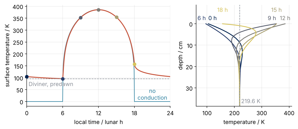
Left: lunar surface temperature in K against local time in lunar hours (one is 29.5 Earth hours). The model stays above the 95 K Diviner line all night, while radiation alone drops to 0 K at sunset. Right: temperature against depth in cm at six times of day; the daily swing dies out within about 30 cm, at 219.6 K.

This is where we end up: on the left the surface through one lunar day, against radiation alone and Diviner's predawn value; on the right the temperature below the ground at six times of day. Six steps build the model, and the last one draws this figure.

Setup

import numpy as np
import matplotlib.pyplot as plt
from scipy.integrate import solve_ivp

# the body: a point on the Moon's equator, Sun overhead at noon; replace these for yours
S = 1361.0                   # sunlight, W/m²
A = 0.12                     # albedo
eps = 0.95                   # emissivity
sigma = 5.670e-8             # Stefan-Boltzmann constant, W/(m² K⁴)
Gamma = 55.0                 # thermal inertia, J/(m² K s^½)
rho, c = 1500.0, 600.0       # density kg/m³ and specific heat J/(kg K), round values
P = 29.53 * 86400            # solar day, noon to noon, s

plt.rcParams.update({                      # the look of every figure below
    "figure.figsize": (7, 3.6), "figure.dpi": 110,
    "axes.spines.top": False, "axes.spines.right": False,
    "axes.grid": True, "grid.alpha": 0.25,
    "font.size": 11, "lines.linewidth": 1.8,
})
INK, ACCENT, SECOND, MUTED = "#1f2a44", "#c8553d", "#2a7f9e", "#8a8f98"

print(f"one lunar day: {P / 86400:.2f} Earth days, {P:.4g} s")

one lunar day: 29.53 Earth days, 2.551e+06 s

Step 1: Balance sunlight against radiation

Start without the ground. If nothing is stored, the surface radiates at every moment what it absorbs, \((1 - A)\,S\max(\cos h, 0) = \varepsilon\sigma T^4\). The code counts time \(t\) from local midnight, so \(h = 2\pi t/P - \pi\), the shifted cosine in absorbed; a lunar hour, a twenty-fourth of the day, is 29.5 Earth hours. The grid holds both midnights, so means skip the last sample.

t = np.linspace(0, P, 481)      # t = 0 at local midnight, 20 samples per lunar hour
hour = 24 * t / P               # local time in lunar hours

def absorbed(t):
    return (1 - A) * S * np.maximum(np.cos(2 * np.pi * t / P - np.pi), 0.0)   # W/m²

T_rad = (absorbed(t) / (eps * sigma)) ** 0.25
print(f"noon maximum {T_rad.max():.1f} K, day mean {T_rad[:-1].mean():.1f} K, "
      f"at 0 K for {100 * np.mean(T_rad[:-1] == 0):.0f} % of the day")

noon maximum 386.2 K, day mean 165.8 K, at 0 K for 50 % of the day

Half the day at absolute zero. Diviner sees nothing of the kind, so heat stored by day must come back up at night: conduction, which the next five steps add. T_rad returns in the final figure as the curve without conduction.

Step 2: Cut the ground into layers

The regolith enters through \(\rho\), \(c\), and \(k\), but the surface feels one combination, the thermal inertia \(\Gamma = \sqrt{k\rho c}\). The code takes \(\Gamma = 55\) in SI units as the input and derives \(k = \Gamma^2/(\rho c)\). The skin depth \(\delta = \sqrt{\kappa P/\pi}\), with \(\kappa = k/(\rho c)\) the diffusivity, is the depth over which a temperature wave of period \(P\) shrinks by a factor of \(e\). In units of \(\delta\) and \(P\) the heat equation has no parameters left, and the conducted flux at the surface is \(\Gamma\sqrt{\pi/P}\) times a derivative in \(z/\delta\). So for constant properties \(\Gamma\) alone sets the surface curve, and \(\rho\) or \(c\) alone only stretches the depths.

The grid follows \(\delta\): the first cell is \(\delta/20\) thick, each one below 15 % thicker, down to 1 m. The top node sits at \(z = 0\), since the surface condition needs the temperature of the surface itself, and each node owns the layer reaching halfway to its neighbors, so the top and bottom layers are half cells. np.r_ joins numbers and arrays into one array:

k = Gamma**2 / (rho * c)        # conductivity, W/(m K)
kappa = k / (rho * c)           # diffusivity, m²/s
skin = np.sqrt(kappa * P / np.pi)

z = np.cumsum(np.r_[0, skin / 20 * 1.15 ** np.arange(60)])
z = np.r_[z[z < 1.0], 1.0]                                  # node depths, m
width = np.diff(np.r_[0.0, (z[:-1] + z[1:]) / 2, 1.0])      # layer thickness of each node, m

print(f"k = {k:.2e} W/(m K), skin depth {100 * skin:.1f} cm, top cell {1000 * z[1]:.2f} mm, "
      f"{z.size} nodes, 1 m = {1 / skin:.1f} skin depths")
with np.printoptions(precision=2, suppress=True):
    print("depth / cm:", 100 * z[:5])
    print("width / cm:", 100 * width[:5])

k = 3.36e-03 W/(m K), skin depth 5.5 cm, top cell 2.75 mm, 30 nodes, 1 m = 18.2 skin depths
depth / cm: [0.   0.28 0.59 0.96 1.37]
width / cm: [0.14 0.3  0.34 0.39 0.45]

Thirty nodes for a meter, fine where the daily wave lives and coarse below. Two checks on the finished model say that is enough: a top cell a quarter as thick moves the surface curve by at most 0.63 K, and a bottom at 15 cm, 2.7 skin depths, would lower the predawn minimum by 2.9 K. At 18.2 skin depths the day does not reach the bottom.

Step 3: Write one ODE per layer: the method of lines

Take one layer, node \(i\) with thickness \(w_i\). Per square meter it holds the heat \(\rho c\,w_i T_i\), and that heat changes only by what flows in at its top minus what flows out at its bottom:

\[ \rho c\,w_i\,\frac{dT_i}{dt} = q_{i-1/2} - q_{i+1/2} . \]

Between two nodes the flux is Fourier's law, \(q = -k\,(T_{i+1} - T_i)/(z_{i+1} - z_i)\), positive downward. Thirty nodes have 31 boundaries, and the flux through the top of layer \(i\), \(q_{i-1/2}\), is q[i] in the code. Two boundaries lie outside the nodes. Through the top one flows the surface condition, absorbed sunlight minus radiation, into the top half layer. Through the bottom one flows nothing, a closed bottom that ignores the Moon's small internal heat flow.

Every node now has its ODE, and the column is a system of 30 of them that solve_ivp integrates like the two of the pendulum. This is the method of lines: time stays continuous, space is cut into lines, one per node. py-pde does this for you and accepts a radiating surface as a boundary expression, but its grids are uniform; the geometric grid of Step 2 is the reason to write rhs by hand.

Before you integrate, test rhs on a column whose answer you know. At one temperature throughout there is no gradient, so every inner flux is zero, and only the top layer, which absorbs and radiates, can change:

def rhs(t, T):
    q = np.r_[0.0, -k * np.diff(T) / np.diff(z), 0.0]   # downward flux through every boundary, W/m²
    q[0] = absorbed(t) - eps * sigma * T[0] ** 4        # the surface
    return (q[:-1] - q[1:]) / (rho * c * width)         # flux in minus flux out

T_flat = np.full(z.size, 250.0)
with np.printoptions(precision=1, suppress=True):
    print("midnight, K/h:", 3600 * rhs(0.0, T_flat)[:4])
    print("noon,     K/h:", 3600 * rhs(P / 2, T_flat)[:4])
print("layers changing:", np.count_nonzero(rhs(0.0, T_flat)), "of", z.size)

midnight, K/h: [-611.3    0.     0.     0. ]
noon,     K/h: [2868.3    0.     0.     0. ]
layers changing: 1 of 30

The prediction holds: 29 of the 30 rates are zero. The top layer cools at 611 K per hour at midnight and warms at 2,868 K per hour at noon, because it is only 1.4 mm thick. That speed is the subject of the next step.

Step 4: Integrate one lunar day with an implicit method

How fast does the top layer settle? Divide its heat capacity per area, \(\rho c\,w_0\), by the rate at which its losses grow with its temperature: \(4\varepsilon\sigma T^3\), the derivative of the radiation, or the conductance \(k/\Delta z\) to the next node. That gives \(\rho c\,w_0/(4\varepsilon\sigma T^3)\) and \(\rho c\,w_0\,\Delta z/k\), minutes both, against a day of 29.5 Earth days.

RK45, the default from the solve_ivp tutorial, is explicit: it builds each step from slopes at states it already knows and stays stable only with steps not much longer than the fastest time scale, all day long. That is stiffness, as in that tutorial's Van der Pol pitfall. BDF, for backward differentiation formulas, is implicit and does the job of the Radau named there: it uses the slope at the new, still unknown state, so each step is an equation for the 30 new temperatures, and its steps can be as long as the solution allows.

BDF solves that equation by Newton's method, which needs the Jacobian, the 30 × 30 table of how each layer's rate responds to each temperature. Without a formula, solve_ivp estimates it by calling rhs about once per layer with one temperature nudged. sol.njev counts these estimates, and by SciPy's convention sol.nfev leaves their calls out, so a wrapper counts every call:

tau_rad = rho * c * width[0] / (4 * eps * sigma * T_rad.max() ** 3)
tau_cond = rho * c * width[0] * z[1] / k
print(f"top layer settles in {tau_rad / 60:.1f} min by radiation at noon, {tau_cond / 60:.1f} min by conduction")

def counted(f):
    def wrapper(t, T):
        wrapper.calls += 1
        return f(t, T)
    wrapper.calls = 0
    return wrapper

calls = {}
for method in ["RK45", "BDF"]:
    f = counted(rhs)
    sol = solve_ivp(f, (0, P), T_flat, method=method, rtol=1e-6, atol=1e-6)
    calls[method], steps = f.calls, sol.t.size - 1
    print(f"{method:4s}  {f.calls:6d} calls   nfev {sol.nfev:6d}   njev {sol.njev:2d}   "
          f"{steps:4d} steps of {P / steps / 60:5.1f} min on average")
print(f"RK45 / BDF: {calls['RK45'] / calls['BDF']:.0f}")
print(f"end of the BDF day: surface {sol.y[0, -1]:.1f} K, bottom {sol.y[-1, -1]:.1f} K, "
      f"predawn minimum {sol.y[0].min():.1f} K")

top layer settles in 1.7 min by radiation at noon, 16.9 min by conduction
RK45   24284 calls   nfev  24284   njev  0   3839 steps of  11.1 min on average
BDF     2125 calls   nfev   1195   njev 30    395 steps of 107.7 min on average
RK45 / BDF: 11
end of the BDF day: surface 107.0 K, bottom 250.0 K, predawn minimum 104.1 K

RK45 takes 3,839 steps of 11 minutes, between the 1.7 and 16.9 minutes of the two time scales, and 24,284 calls. BDF takes 395 steps of nearly two hours and 2,125 calls, a factor of 11 fewer, of which nfev shows only 1,195: 30 Jacobian estimates of 31 calls each are missing. And the day does not close on itself: it started at 250 K throughout and ends at 107.0 K on top, still 250.0 K at the bottom.

Step 5: Spin up to a periodic day

The answer is the day that repeats: start each day where the last one ended until two days agree. That is slow at the bottom, where a change at the surface reaches depth \(L\) on the time scale \(L^2/\kappa\), 105 lunar days for 1 m. The shortcut is to average the heat equation over one periodic day. The left side averages to zero, since \(T\) returns to its start, so the mean \(\langle T\rangle\) is linear in \(z\), and with no flux at the bottom it is constant: the day-mean temperature is the same at every depth.

So after each day the loop shifts the whole column until the bottom, whose temperature hardly moves within a day, sits at the day's mean surface temperature. A constant added to every layer leaves every conducted flux unchanged; only the radiation of the surface responds, and the top layer readjusts within the minutes of Step 4. The loop stops when two surface curves agree to 0.01 K:

print(f"the bottom forgets the start after about (1 m)²/κ = {1.0**2 / kappa / P:.0f} lunar days")

T, previous = T_flat, np.full(t.size, 250.0)      # the start, as a column and as a surface curve
for day in range(1, 100):
    sol = solve_ivp(rhs, (0, P), T, method="BDF", t_eval=t, rtol=1e-6, atol=1e-6)
    T = sol.y[:, -1] + sol.y[0, :-1].mean() - sol.y[-1, -1]       # the shift
    change = np.abs(sol.y[0] - previous).max()
    print(f"day {day:2d}   surface curve moved {change:7.3f} K   bottom {sol.y[-1, -1]:5.1f} K, shifted to {T[-1]:5.1f} K")
    if change < 0.01:
        break
    previous = sol.y[0]

Ts, deep = sol.y[0], sol.y[-1, -1]
print(f"periodic after {day} lunar days: mean surface {Ts[:-1].mean():.1f} K, at 1 m {deep:.1f} K")

the bottom forgets the start after about (1 m)²/κ = 105 lunar days
day  1   surface curve moved 145.939 K   bottom 250.0 K, shifted to 224.7 K
day  2   surface curve moved 168.363 K   bottom 224.7 K, shifted to 218.4 K
day  3   surface curve moved  16.574 K   bottom 218.4 K, shifted to 219.1 K
day  4   surface curve moved   6.803 K   bottom 219.0 K, shifted to 219.6 K
day  5   surface curve moved   0.214 K   bottom 219.5 K, shifted to 219.6 K
day  6   surface curve moved   0.304 K   bottom 219.6 K, shifted to 219.6 K
day  7   surface curve moved   0.032 K   bottom 219.6 K, shifted to 219.7 K
day  8   surface curve moved   0.035 K   bottom 219.6 K, shifted to 219.7 K
day  9   surface curve moved   0.019 K   bottom 219.6 K, shifted to 219.7 K
day 10   surface curve moved   0.013 K   bottom 219.6 K, shifted to 219.7 K
day 11   surface curve moved   0.009 K   bottom 219.6 K, shifted to 219.7 K
periodic after 11 lunar days: mean surface 219.7 K, at 1 m 219.6 K

The first shift alone takes the bottom from 250.0 to 224.7 K, and after 11 days instead of a hundred the column agrees with the argument: 219.7 K mean at the surface, 219.6 K at 1 m. The argument assumes constant properties and a closed bottom; with a conductivity that grows with temperature (Variations) or heat from the interior, the shift aims at the wrong temperature. Pitfall 1 shows the loop without the shift.

Step 6: Compare with the Moon and draw the day and the depth profiles

The last day of the loop is the answer. The code prints what Diviner and the Apollo probes can check and draws the surface through the day and the profiles below it at six local times, in the cividis colormap from dark at midnight to light at sunset:

print(f"noon maximum {Ts.max():.1f} K, at sunset {Ts[20 * 18]:.1f} K")
# specific to the Moon: the measured values in this print, the 95 K line, the hand-placed hour labels
print(f"predawn {Ts.min():.1f} K (Diviner about 95 K), at 1 m {deep:.1f} K (Apollo 15 and 17 about 250 K)")

fig, (ax1, ax2) = plt.subplots(1, 2, figsize=(8, 3.4), width_ratios=[3, 2], layout="constrained")
ax1.plot(hour, T_rad, color=SECOND, lw=1.1)
ax1.plot(hour, Ts, color=ACCENT, lw=1.8)
ax1.axhline(95, color=MUTED, ls="--", lw=1)
ax1.text(0.3, 88, "Diviner, predawn", color=MUTED, va="top")
ax1.text(21, 8, "no\nconduction", color=SECOND, ha="center")
ax1.set(xlabel="local time / lunar h", ylabel="surface temperature / K", xticks=range(0, 25, 6), xlim=(0, 24))
for i, (h, ha, y) in enumerate([(0, "left", -0.2), (6, "right", -0.2), (9, "right", -0.2),
                                (12, "center", -0.2), (15, "center", -0.9), (18, "center", -0.9)]):
    color = plt.cm.cividis(0.85 * i / 5)             # dark to light through the day, short of the palest yellow
    ax1.plot(h, Ts[20 * h], "o", color=color, ms=6, zorder=3, clip_on=False)
    ax2.plot(sol.y[:, 20 * h], 100 * z, color=color, lw=1.6)
    ax2.text(sol.y[0, 20 * h], 100 * skin * y, f"{h} h", color=color, ha=ha, va="bottom")
ax2.axvline(deep, color=MUTED, ls="--", lw=1)
ax2.text(deep + 5, 0.03, f"{deep:.1f} K", color=MUTED, transform=ax2.get_xaxis_transform())
ax2.set(xlabel="temperature / K", ylabel="depth / cm", ylim=(700 * skin, -160 * skin), xlim=(Ts.min() - 35, Ts.max() + 25))
plt.show()

noon maximum 385.3 K, at sunset 156.7 K
predawn 95.6 K (Diviner about 95 K), at 1 m 219.6 K (Apollo 15 and 17 about 250 K)

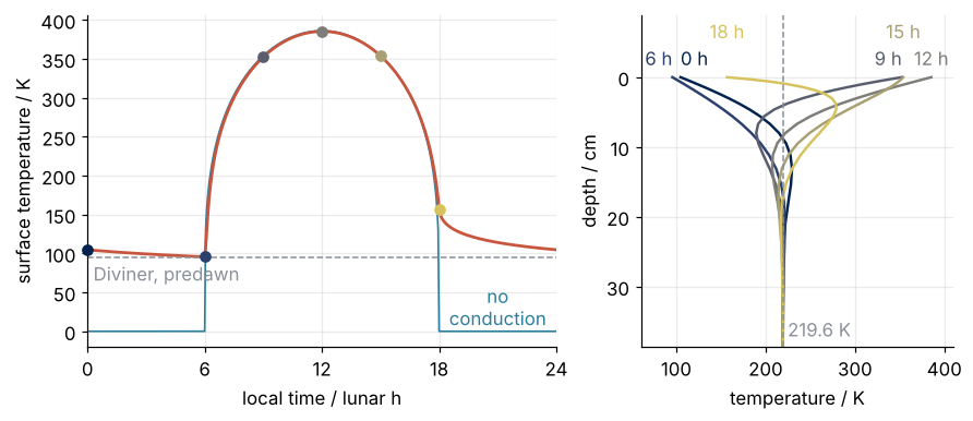
Left: lunar surface temperature in K against local time in lunar hours (one is 29.5 Earth hours). The model stays above the 95 K Diviner line all night, while radiation alone drops to 0 K at sunset. Right: temperature against depth in cm at six times of day; the daily swing dies out within about 30 cm, at 219.6 K.

The surface curve is the part to trust. Its predawn minimum of 95.6 K agrees with the about 95 K that Diviner measures at the equator, and \(\Gamma = 55\) is taken from Hayne et al. (2017), not fitted: \(\Gamma = 30\) would give 82.8 K and \(\Gamma = 80\) 104.4 K. At sunset the ground holds the surface at 156.7 K, where radiation alone gives 0 K.

The deep temperature is 30 K below the about 250 K that the Apollo 15 and 17 heat flow probes read at 1 m, and since they sit at 26°N and 20°N, the gap at the equator is larger. With constant properties the deep temperature must equal the mean surface temperature (Step 5). Real regolith conducts better when hot, through radiation between its grains, and is denser below a few centimeters. Tuning \(\Gamma\) to hit both numbers would hide where the constant-property model ends; the last of the variations closes part of the gap instead.

Pitfalls

Two days that agree and a deep temperature that is still wrong. Replace the shift line by T = sol.y[:, -1], and the run from 250 K stops after 35 lunar days with two days agreeing to 0.01 K. The predawn minimum is only 0.4 K off, but the bottom sits at 236.8 K, 17.2 K too warm. The column needs about 105 lunar days to arrive, and long before that each day moves the surface by less than the stop test can see. Keep the shift, and before you trust any spin-up, compare the bottom with the mean surface temperature.

A uniform grid. With 32 evenly spaced nodes the cells are 3.2 cm thick, more than half a skin depth, and the predawn minimum comes out only 0.5 K low, which looks like success. The error sits at sunrise: the thick top layer warms too slowly, and at 6.2 h the surface is 29.9 K too cold. An even grid at the 2.75 mm of the top cell needs 364 nodes for the same meter, twelve times the 30 of the geometric grid. When you test a grid, compare the whole curve, not one number.

The default method. Leave out method="BDF" and solve_ivp runs RK45 without a word of complaint. On this grid it is only slow, but refine the top cell and it gets worse quickly: with the top cell halved, RK45 needs 65,816 calls of rhs against 2,276 for BDF, a factor of 29 where it was 11, while BDF hardly notices. The fast time scale shrinks with the top layer, and the explicit steps shrink with it. A run that took a second and takes a minute after you refined the grid is the symptom. Use BDF or Radau, as in the stiffness pitfall of the solve_ivp tutorial. Compare methods by counted calls, not by nfev: the Jacobian estimates add 78 % to the nfev of BDF in Step 4, against 5 % for Radau on that tutorial's Van der Pol oscillator, whose factor of forty stands.

Variations

Mercury. Set \(S\), \(A\), \(\varepsilon\), and \(\Gamma\) for Mercury and \(P\) = 176 Earth days, the solar day, not the 58.6-day rotation. A fixed \(S\) is itself an approximation there, since Mercury's distance from the Sun changes by a factor of about 1.5 around its orbit, so make it a function of \(t\).
An asteroid. The skin depth grows as \(\sqrt{P}\), so a 6-hour day on regolith like the Moon's brings it down from 5.5 cm to 5 mm, and a rockier, larger \(\Gamma\) raises it again. The grid follows \(\delta\) by itself; the one change is the bottom, at about 20 skin depths instead of 1 m.
Another latitude. Multiply absorbed by \(\cos\varphi\), for a body without axial tilt, which the Moon nearly is. The Apollo 15 site is at \(\varphi\) = 26°.
Conductivity that grows with temperature. Hayne et al. (2017) use \(k(T) = k_c\,(1 + \chi\,(T/350\ \mathrm{K})^3)\); evaluate it between neighbors in the flux line of rhs. The hot day then conducts heat down better than the cold night conducts it back up, so the deep temperature rises above the mean surface temperature, which closes part of the gap of Step 6, and \(\Gamma\) no longer sets the curve alone. The shift of Step 5 then aims too low: aim it at the bottom temperature \(T_b\) with \(U(T_b) = \langle U(T_0)\rangle\), where \(U(T) = \int k\,dT\).

Cheat sheet

skin = np.sqrt(k / (rho * c) * P / np.pi)                      # depth of the daily temperature wave
z = np.cumsum(np.r_[0, skin / 20 * 1.15 ** np.arange(60)])     # top cell skin/20, growing by 15 %
z = np.r_[z[z < L], L]                                         # node depths from 0 to the bottom L
width = np.diff(np.r_[0.0, (z[:-1] + z[1:]) / 2, L])           # each node's layer; half cells at both ends
def rhs(t, T):
    q = np.r_[0.0, -k * np.diff(T) / np.diff(z), 0.0]          # Fourier's law between nodes, positive down
    q[0] = absorbed(t) - eps * sigma * T[0] ** 4               # radiating surface; q[-1] = 0 closes the bottom
    return (q[:-1] - q[1:]) / (rho * c * width)                # flux in minus flux out
sol = solve_ivp(rhs, (0, P), T, method="BDF", t_eval=t, rtol=1e-6, atol=1e-6)   # implicit: the column is stiff
T = sol.y[:, -1] + sol.y[0, :-1].mean() - sol.y[-1, -1]       # spin-up shift; holds for constant k, closed bottom