py-pde from the ground up: the heat equation on a square plate

The problem: how long does a plate take to forget its start?

A square plate of side 1 sits at temperature 0. At t = 0 you clamp its left edge at 1 and its right edge at 0, and you insulate the top and bottom. Heat then spreads by the heat equation,

\[\frac{\partial T}{\partial t} = D\,\nabla^2 T ,\]

with diffusivity \(D = 0.1\) and \(\nabla^2 = \partial_x^2 + \partial_y^2\) the Laplacian, the sum of the second derivatives. Where the plate ends up needs no computer. Once nothing changes, \(\nabla^2 T = 0\), nothing varies along y, and the temperature is the straight line \(T = 1 - x\). How long it takes to get there is the real question, and py-pde, a Python package that solves PDEs on grids by finite differences, answers it with numbers: at t = 1 the plate is still 0.24 off the line at its worst point, at t = 20 the gap is 1.7 × 10⁻⁹. A solute soaking into a gel slab, or a dopant diffusing into silicon, obeys the same equation with a different D.

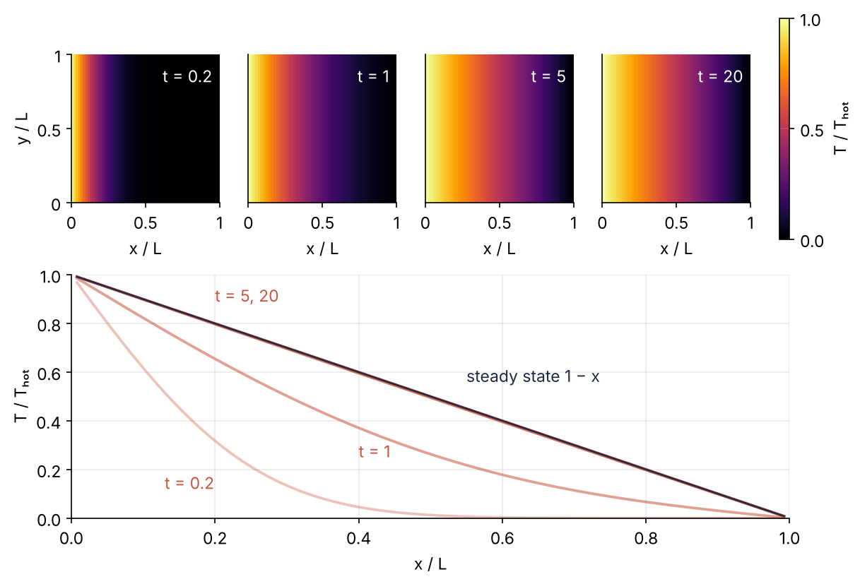
Top: temperature of a square plate whose left edge is held at 1 and right edge at 0, at t = 0.2, 1, 5 and 20. Bottom: the temperature along the midline at the same times against the straight line 1 − x. By t = 20 the profile lies on the line.

The top row is the plate at four times, the bottom row the temperature along its midline against the straight line, both in units of the hot edge's temperature, \(T_\text{hot}\). All of it comes from one solve call that keeps the field at the times you ask for, and Step 6 draws it.

Setup

py-pde installs with pip install py-pde and imports as pde.

import numpy as np
import matplotlib.pyplot as plt
import pde

L = 1.0    # side of the plate
D = 0.1    # diffusivity, length^2 per time unit

plt.rcParams.update({                      # the look of every figure below
    "figure.figsize": (8, 5.4), "figure.dpi": 110,
    "axes.spines.top": False, "axes.spines.right": False,
    "axes.grid": True, "grid.alpha": 0.25,
    "font.size": 11, "lines.linewidth": 1.8,
})
INK, ACCENT, SECOND, MUTED = "#1f2a44", "#c8553d", "#2a7f9e", "#8a8f98"

print(f"diffusion time L^2/D = {L**2 / D:g}")

diffusion time L^2/D = 10

Step 1: Lay out the grid and the starting field

py-pde keeps the space apart from what lives on it. A CartesianGrid is the space, a rectangle cut into cells, and a ScalarField is one number per cell. Sixty-four cells per side:

grid = pde.CartesianGrid([[0, L], [0, L]], 64)
T0 = pde.ScalarField(grid, 0.0)

print("cell size:", grid.discretization)
print(T0.data.shape, grid.axes_coords[0][:3])

cell size: [0.015625 0.015625]
(64, 64) [0.0078125 0.0234375 0.0390625]

The first coordinate is not 0 but half a cell in. py-pde stores values at cell centers, so the edges of the plate are not in the array at all, and what happens there is set by the boundary conditions. T0.data is a plain NumPy array indexed [x, y], the first index running along x. The answer here will not depend on y, because every edge is uniform along its length. Heat only part of an edge and y matters, so the plate stays 2D; here the missing y dependence is a free check in Step 4.

py-pde knows no units. The bounds are in whatever length unit you choose, and D must be in that unit squared per time unit; Pitfall 3 shows what a mismatch does.

Step 2: State the boundary conditions in one dictionary

The four edges go into one dictionary, keyed by where they are:

bc = {"x-": {"value": 1}, "x+": {"value": 0}, "y": {"derivative": 0}}
eq = pde.DiffusionPDE(diffusivity=D, bc=bc)
print(eq.expression)

0.1 * ∇²(c)

x- is the lower end of the x axis, the left edge, and x+ the upper end. y alone sets both y edges; y- and y+ exist for when they differ. value holds the temperature on the edge fixed (a Dirichlet condition). derivative fixes \(\partial T/\partial n\), the derivative along the outward normal (a Neumann condition). Zero means no heat crosses: an insulated edge. The printed expression is the equation py-pde will integrate, with the field called c because DiffusionPDE is written for any diffusing quantity.

A nonzero derivative is a heat flux, and its sign is where people go wrong. By Fourier's law the heat flux leaving through an edge is \(-k\,\partial T/\partial n\), with \(k\) the thermal conductivity. A flux \(q\) flowing into the plate is therefore {"derivative": q / k} on whichever edge: positive heats, negative cools. Step 5 runs one.

Step 3: Integrate with a time step you chose

First, what py-pde does with the equation. Put a 1 into one cell, apply the Laplacian, and multiply by \(\Delta x^2\):

dx = grid.discretization[0]
spike = pde.ScalarField(grid, 0.0)
spike.data[32, 32] = 1
print((spike.laplace(bc).data * dx**2)[31:34, 31:34])

[[ 0.  1.  0.]
 [ 1. -4.  1.]
 [ 0.  1.  0.]]

Every cell gets the sum of its four neighbors minus four times itself, over \(\Delta x^2\). That turns the PDE into 4,096 coupled ODEs, one per cell, the method of lines: the kind of system solve_ivp from the ground up integrates, only larger. The default solver steps them with explicit Euler, \(T_\text{new} = T + \Delta t\,D\,\nabla^2 T\), which gives the cell's own old value the weight \(1 - 4D\,\Delta t/\Delta x^2\). Let that weight go negative and a cell above its neighbors overshoots below them, overshoots back on the next step, and a checkerboard grows: that is what unstable means here. Keeping it non-negative gives \(\Delta t \le \Delta x^2/(4D)\). On a line, with two neighbors, the limit is \(\Delta x^2/(2D)\).

The run below brings two additions. A MemoryStorage keeps fields, and its tracker stops the run at the listed times to hand it a copy. ret_info=True also returns a dictionary whose "solver" entry says what stepped and how often:

dt_max = dx**2 / (4 * D)
dt = 5e-4
print(f"dt_max = {dt_max:.1e}, dt = {dt:.0e} ({dt / dt_max:.2f} of the limit)")

storage = pde.MemoryStorage()
T_end, info = eq.solve(T0, t_range=20, dt=dt, ret_info=True,
                       tracker=storage.tracker([0.2, 1, 5, 20]))
s = info["solver"]
print(s["class"], s["steps"], s["dt"], "adaptive:", s["dt_adaptive"])
print("stored at t =", storage.times)

dt_max = 6.1e-04, dt = 5e-04 (0.82 of the limit)
EulerSolver 40000 0.0005 adaptive: False
stored at t = [0.2, 1.0, 5.0, 20.0]

That is 40,000 fixed steps, and the field at exactly the four times listed. Any tracker you pass replaces the default ones, a progress bar and a stop once the field is no longer finite. The first call takes 10 to 15 s while numba, a compiler py-pde uses, translates the loop to machine code. Leave out dt and py-pde adapts the step itself. Pass it, and stability is your job: stay a little under the limit, as the 0.82 here does.

Step 4: Check the result against the straight line

Steady means \(\partial T/\partial t = 0\), so \(\nabla^2 T = 0\). Nothing depends on y, which leaves \(T'' = 0\) with \(T = 1\) at the left edge and \(T = 0\) at the right: the line \(T = 1 - x/L\). How fast the plate gets there follows from the lecture too: what is left, \(T - (1 - x/L)\), is zero at both held edges, and separation of variables makes it a sum of sines \(\sin(n\pi x/L)\), each decaying as \(e^{-n^2\pi^2 D t/L^2}\). Soon only the slowest is left, the half sine with \(n = 1\). Its rate \(\pi^2 D/L^2\) is \(\pi^2\) over the diffusion time \(L^2/D = 10\), a factor e per time unit to a good approximation.

The cell compares each stored field with the line, predicts t = 20 from t = 5, and checks the spread along y. exact[:, None] turns the profile into a column, so it is compared with every y at once, and np.ptp ("peak to peak") is max minus min:

x = grid.axes_coords[0]
exact = 1 - x / L

deviation = {}
for t, field in storage.items():
    deviation[t] = np.abs(field.data - exact[:, None]).max()
    print(f"t = {t:4g}   max |T - (1 - x)| = {deviation[t]:.3g}")

rate = np.pi**2 * D / L**2
print(f"predicted at t = 20 from t = 5: {deviation[5] * np.exp(-rate * 15):.2g}")
print("largest spread along y:", np.ptp(T_end.data, axis=1).max())

t =  0.2   max |T - (1 - x)| = 0.571
t =    1   max |T - (1 - x)| = 0.238
t =    5   max |T - (1 - x)| = 0.00458
t =   20   max |T - (1 - x)| = 1.7e-09
predicted at t = 20 from t = 5: 1.7e-09
largest spread along y: 0.0

At t = 1 a picture already looks like a ramp, and it is off by 0.24. From the 0.0046 at t = 5, the half sine alone predicts the 1.7 × 10⁻⁹ printed at t = 20. Run to several \(L^2/D\) before you call anything steady, and check against a case you can solve. The spread along y is exactly zero, as it must be.

Step 5: Feed heat through an edge instead of holding it hot

Now a heater on the left edge pushes in a fixed flux, \(q/k = 1\) in the plate's units. There the outward normal points along −x, so derivative 1 means \(\partial T/\partial x = -1\), the slope of \(1 - x\), and the cold right edge pins the line at 0. The steady state is the same line. Run it in the same session as Step 3 and something odd comes back:

bc_flux = {"x-": {"derivative": 1}, "x+": {"value": 0}, "y": {"derivative": 0}}
eq_flux = pde.DiffusionPDE(diffusivity=D, bc=bc_flux)

T_flux = eq_flux.solve(T0, t_range=20, dt=dt, tracker=None)
print(f"t = 20   max |T - (1 - x)| = {np.abs(T_flux.data - exact[:, None]).max():.3g}")

t = 20   max |T - (1 - x)| = 1.7e-09

That is Step 4's number to the last digit, because it is Step 4's run. py-pde 0.59.0 caches the compiled operator under a key that sees the same grid, edge, and number 1, but not that one is a value and the other a derivative. A run that differs from an earlier one only in the type of a condition needs a fresh Python session or backend="numpy", which compiles nothing and is slower.

The deviation now has zero slope at the flux edge, where \(T\) and the line obey the same condition. Its slowest mode is then the quarter cosine \(\cos(\pi x/2L)\), which decays at \(\pi^2 D/(4L^2) = 0.25\) per time unit, a quarter of Step 4's rate. The cell predicts t = 50 from t = 20 with it:

storage_flux = pde.MemoryStorage()
eq_flux.solve(T0, t_range=50, dt=dt, backend="numpy",
              tracker=storage_flux.tracker([20, 50]))

dev_flux = {t: np.abs(f.data - exact[:, None]).max() for t, f in storage_flux.items()}
for t, d in dev_flux.items():
    print(f"t = {t:4g}   max |T - (1 - x)| = {d:.3g}")
print(f"predicted at t = 50 from t = 20: {dev_flux[20] * np.exp(-rate / 4 * 30):.3g}")

t =   20   max |T - (1 - x)| = 0.00583
t =   50   max |T - (1 - x)| = 3.55e-06
predicted at t = 50 from t = 20: 3.55e-06

At t = 20 the plate is still 0.0058 off the line, where the held edge had reached 1.7 × 10⁻⁹. The quarter cosine predicts the 3.55 × 10⁻⁶ at t = 50 exactly. The clock depends on the edges, not only on \(L^2/D\).

Step 6: Draw the field and the midline profile

py-pde draws a field into axes you hand it with ax=, so the style of the setup applies. vmin and vmax give the four panels one color scale, and inferno is a perceptually uniform colormap that reads as temperature. slice does not interpolate: it returns the row of cells nearest to y = 0.5, centered at y = 0.492, the same thing on a plate where nothing varies along y. plot returns a reference whose element is the Matplotlib image the colorbar needs, and action="none" leaves the figure alone once the panel is drawn:

fig = plt.figure(layout="constrained")
fig.get_layout_engine().set(wspace=0.12)       # room between neighboring tick labels
gs = fig.add_gridspec(2, 5, height_ratios=[1, 1.1], width_ratios=[1, 1, 1, 1, 0.07])
ax_p = fig.add_subplot(gs[1, :])

for i, (t, field) in enumerate(storage.items()):
    ax = fig.add_subplot(gs[0, i])
    im = field.plot(kind="image", ax=ax, cmap="inferno", vmin=0, vmax=1,
                    colorbar=False, title="", action="none")
    ax.set(xlabel="x / L", ylabel="y / L" if i == 0 else "",
           xticks=[0, 0.5, 1], xticklabels=["0", "0.5", "1"],
           yticks=[0, 0.5, 1] if i == 0 else [],
           yticklabels=["0", "0.5", "1"] if i == 0 else [])
    ax.grid(False)
    ax.text(0.95, 0.92, f"t = {t:g}", transform=ax.transAxes,
            ha="right", va="top", color="white")
    ax_p.plot(x, field.slice({"y": 0.5}).data, color=ACCENT,
              alpha=[0.35, 0.55, 0.8, 1.0][i])

fig.colorbar(im.element, cax=fig.add_subplot(gs[0, 4]), label="T / Tₕₒₜ", ticks=[0, 0.5, 1])
ax_p.plot(x, exact, color=INK, lw=1.2, zorder=3)
ax_p.text(0.55, 0.56, "steady state 1 − x", color=INK)
ax_p.text(0.13, 0.12, "t = 0.2", color=ACCENT)
ax_p.text(0.40, 0.25, "t = 1", color=ACCENT)
ax_p.text(0.20, 0.89, "t = 5, 20", color=ACCENT)
ax_p.set(xlabel="x / L", ylabel="T / Tₕₒₜ", xlim=(0, 1), ylim=(0, 1))
plt.show()

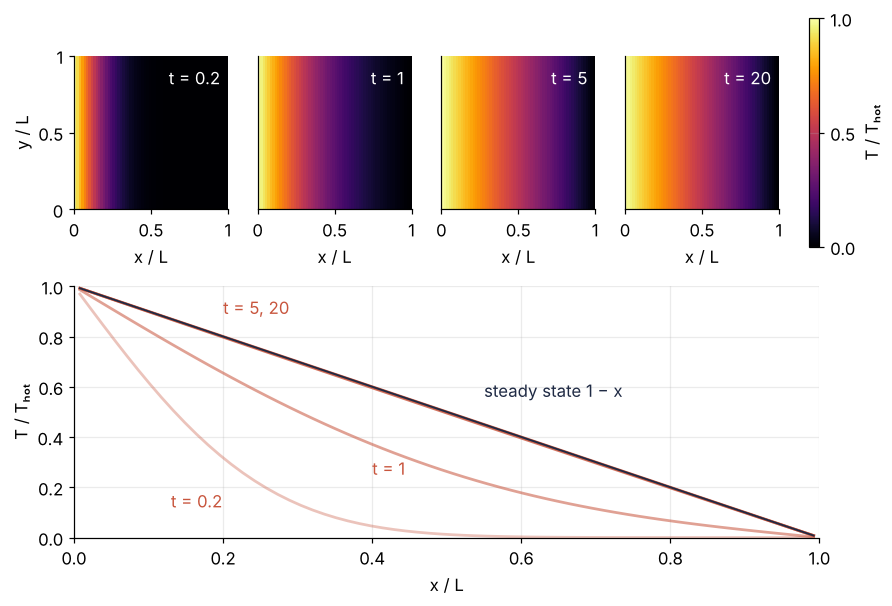
The front enters from the left and fills the plate within a few time units. By t = 5 the profile lies on the line to the eye, and Step 4's 0.0046 says how far off it still is.

Pitfalls

A time step that worked on the coarse grid. You refine to 128 cells per side for a sharper picture and keep the step:

grid128 = pde.CartesianGrid([[0, L], [0, L]], 128)
T128 = eq.solve(pde.ScalarField(grid128, 0.0), t_range=0.05, dt=dt, tracker=None)
print(f"largest |T| after 100 steps: {np.abs(T128.data).max():.1e}")
print("signs along a row:", np.sign(T128.data[:8, 64]))

largest |T| after 100 steps: 2.5e+34
signs along a row: [-1.  1. -1.  1. -1.  1. -1.  1.]

Halving \(\Delta x\) quarters the limit, to 1.5 × 10⁻⁴, so the step is 3.3 times too large. The weight of Step 3 is negative, and the checkerboard, alternating from cell to cell, has reached 10³⁴ after 100 steps. Compute dt from the grid every time, or leave it out. This plate is more forgiving than the formula: with nothing varying along y it only feels the line limit, so on the 64 grid it tolerates up to twice \(\Delta x^2/(4D)\). A field that varies in both directions does not.

A boundary dictionary that says less than you think. {"x": {"value": 1}, ...} sets both x edges, and the plate heats to 1 everywhere. Giving x- without x+ fails with a message that names neither the missing edge nor the fix:

try:
    pde.DiffusionPDE(diffusivity=D, bc={"x-": {"value": 1}, "y": {"derivative": 0}}).solve(
        T0, t_range=1, dt=dt, tracker=None)
except Exception as err:
    print(f"{type(err).__name__}: {str(err).split('.')[0]}")

BCDataError: Boundary condition `auto_periodic_neumann` not defined

Leaving out the y entry raises nothing at all: the y edges silently become insulated, which is right here and wrong as soon as you meant something else. Name all four edges, x-, x+, y-, y+.

Units that do not match. The symptom is a run that seems frozen, or one that is over after the first step. Take a gel slab 2 mm thick and a solute with D of order 10⁻⁹ m²/s. With the grid in millimeters and D left in m²/s, \(L^2/D\) is 4 × 10⁹ s, and nothing moves in any t_range you would think of. Converted, D is 10⁻³ mm²/s and \(L^2/D\) is 4,000 s, about an hour. Use one unit system and check t_range against \(L^2/D\), the clock of Step 4. Left in m²/s, that clock reads 127 years, a long wait for a gel.

Variations

FiPy. The same plate in finite volumes, which balance the heat crossing each cell face, with NIST's package. The equation becomes TransientTerm() == DiffusionTerm(coeff=D), and the edge temperatures become constrain calls on the faces.
scikit-fem. A plate that is not a rectangle, say an L shape (MeshTri.init_lshaped()). A finite-element mesh of triangles fitted to the shape replaces the grid, and the steady state is one sparse solve, a linear system with mostly zero entries.
findiff. The steady state alone. PDE(Diff(0, dx)**2 + Diff(1, dy)**2, rhs, bcs) turns \(\nabla^2 T = 0\) with the four edge conditions into one linear system: no time stepping, no step limit.
Reaction and diffusion. pde.PDE({"c": "0.1 * laplace(c) + c - c**3"}, bc=bc) adds a reaction term on the same grid with the same dictionary, which gives the Allen-Cahn equation, a model of two phases separating. The same PDE class takes systems of several fields.

Cheat sheet

grid = pde.CartesianGrid([[0, Lx], [0, Ly]], [nx, ny])       # bounds in your length unit
T0 = pde.ScalarField(grid, 0.0)                              # values at cell centers, data[x, y]
bc = {"x-": {"value": 1}, "x+": {"derivative": q / k},      # fixed T; heat flux q flowing in
      "y-": {"derivative": 0}, "y+": {"derivative": 0}}      # dT/dn outward; 0 means insulated
eq = pde.DiffusionPDE(diffusivity=D, bc=bc)                  # dT/dt = D laplace(T)
dt = 0.8 * min(grid.discretization)**2 / (4 * D)             # explicit Euler limit in 2D
storage = pde.MemoryStorage()
T, info = eq.solve(T0, t_range=t_end, dt=dt, ret_info=True,  # omit dt: adaptive step
                   tracker=storage.tracker([t1, t2]))        # keep the field at t1, t2
profile = T.slice({"y": y0}).data                            # the row of cells nearest y0