The Fisher matrix: how well a supernova survey will measure dark energy (Python)

The question

A planned survey will find 1,000 type Ia supernovae with redshifts between 0.1 and 1.5 and measure the distance to each with an error of 0.15 mag. Before anyone grants it years of telescope time, one question has to be answered: will it measure w, the equation of state of dark energy, to ± 0.1, or only to ± 0.3? The Fisher matrix answers that before the first night, from the model and the error bars alone.

The distance an astronomer reads off a supernova's apparent brightness is the distance modulus μ, a logarithm of the luminosity distance \(d_L\) of Cosmological distances with quad. How \(d_L\) grows with redshift z depends on what the universe is made of. In a flat universe a share Ωm of the energy is matter and the rest is dark energy, whose pressure is \(p = w\rho c^2\), w times its energy density. For w = −1, Einstein's cosmological constant, that density never thins out as space expands, and any other value would be news. The model the survey will fit is

\[\mu(z) = 5\log_{10}\frac{d_L(z)}{10\ \mathrm{pc}} + \Delta M, \qquad d_L(z) = (1+z)\,\frac{c}{H_0}\int_0^z \frac{dz'}{E(z')}, \qquad E(z) = \sqrt{\Omega_m (1+z)^3 + (1-\Omega_m)(1+z)^{3(1+w)}} .\]

ΔM is the unknown offset in the supernovae's true brightness, a nuisance parameter: nobody wants it, everybody has to fit it. It also absorbs the Hubble constant \(H_0\), which enters μ only in the combination \(\Delta M - 5\log_{10} H_0\), so \(H_0\) stays fixed at 70 km/s/Mpc.

Show code

import numpy as np
import matplotlib.pyplot as plt
import matplotlib.patheffects as pe
from scipy.integrate import quad
from scipy.interpolate import CubicSpline
from scipy.optimize import brentq, curve_fit, least_squares

plt.rcParams.update({
    "figure.figsize": (7, 3.6), "figure.dpi": 110,
    "axes.spines.top": False, "axes.spines.right": False,
    "axes.grid": True, "grid.alpha": 0.25,
    "font.size": 11, "lines.linewidth": 1.8,
})
INK, ACCENT, SECOND, MUTED = "#1f2a44", "#c8553d", "#2a7f9e", "#8a8f98"

C_KMS, H0 = 299_792.458, 70.0            # km/s, km/s/Mpc
SIGMA, N = 0.15, 1000                    # mag per supernova, supernovae
p_fid = np.array([0.3, -1.0, 0.0])       # Omega_m, w, Delta M
rng = np.random.default_rng(244)
z = np.sort(rng.uniform(0.1, 1.5, N))    # the survey's design, drawn once

z_grid = np.linspace(0, 1.5, 151)


def E(zp, Om, w):
    return np.sqrt(Om * (1 + zp) ** 3 + (1 - Om) * (1 + zp) ** (3 * (1 + w)))


def mu(z, Om, w, dM):
    """Distance modulus / mag. quad on 150 short pieces, summed, then a spline to the supernovae:
    one quad per supernova would make the 500 fits below take ten minutes."""
    pieces = [quad(lambda x: 1 / E(x, Om, w), a, b, epsabs=0, epsrel=1e-12)[0]
              for a, b in zip(z_grid[:-1], z_grid[1:])]
    D = CubicSpline(z_grid, np.concatenate([[0.0], np.cumsum(pieces)]))(z)
    d_L = (1 + z) * C_KMS / H0 * D       # Mpc
    return 5 * np.log10(d_L) + 25 + dM   # 5 log10(d_L / 10 pc)


mu_fid = mu(z, *p_fid)
mu_obs = mu_fid + SIGMA * rng.standard_normal(N)       # one simulated survey
shift = mu(z, 0.3, -0.9, 0.0) - mu_fid

fig, (ax1, ax2) = plt.subplots(2, 1, figsize=(7, 4.6), sharex=True, height_ratios=[1.6, 1])
ax1.errorbar(z, mu_obs, yerr=SIGMA, fmt="o", ms=2, lw=0.6, color=INK, alpha=0.3)
ax1.plot(z, mu_fid, color=INK, path_effects=[pe.withStroke(linewidth=4, foreground="white")])
k = np.searchsorted(z, 0.4)
ax1.annotate("model at Ωm = 0.3, w = −1, ΔM = 0", xy=(z[k], mu_fid[k]), xytext=(0.12, 45.6), color=INK,
             va="top", arrowprops=dict(arrowstyle="-", color=INK, lw=1, shrinkB=0))
ax1.set(ylabel="μ / mag")
ax2.axhspan(-SIGMA, SIGMA, color=MUTED, alpha=0.15, lw=0)
ax2.axhline(0, color=MUTED, lw=1, ls="--")
ax2.plot(z, shift, color=SECOND)
ax2.text(0.12, 0.11, "error of one supernova, ±0.15 mag", color=MUTED, va="center")
ax2.text(1.48, shift[-1] - 0.025, f"w = −0.9: largest shift {np.abs(shift).max():.3f} mag",
         color=SECOND, ha="right", va="top")
ax2.set(xlabel="z", ylabel="Δμ / mag", xlim=(0.05, 1.52), ylim=(-0.19, 0.19))
plt.show()

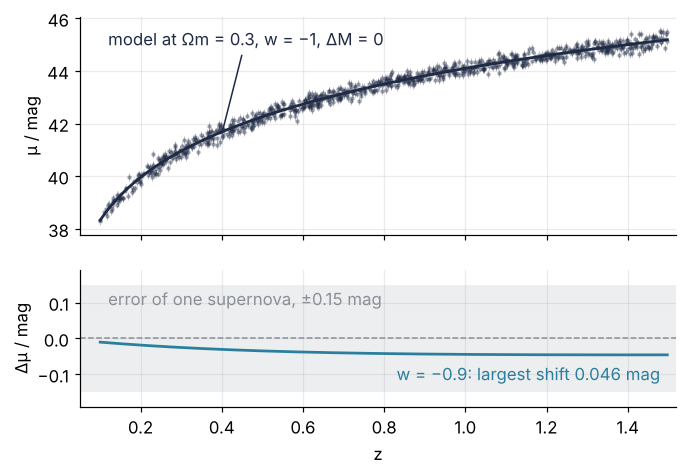
Top: distance modulus μ in mag against redshift z for 1,000 simulated supernovae with error bars of 0.15 mag, and the model curve. Bottom: the shift of μ when w goes from −1 to −0.9 with Ωm and ΔM held, at most 0.046 mag, well inside the shaded ±0.15 mag error of one supernova.

The top panel is one simulated survey at Ωm = 0.3, w = −1, ΔM = 0. The bottom panel is what a 10 % change in w does: at w = −0.9, with Ωm and ΔM held, the curve moves by at most 0.046 mag, less than a third of one supernova's error bar.

Two things are obvious. No single supernova can see the change, and 1,000 of them average their noise down, so together they might. Less obvious: how well can the survey measure w before the data exist, and why should the answer depend on Ωm and the offset, two numbers nobody asked about?

The idea: how fast the fit gets worse

Take the survey without noise, the curve μ(z) at the fiducial values Ωm = 0.3, w = −1, ΔM = 0, and score other models against it with the χ² of Least squares: the misses, each divided by the error bar of 0.15 mag, squared and summed over the 1,000 supernovae. At the fiducial values χ² is zero. Move w away and it rises, and how fast it rises is how much the survey knows about w.

There are two ways to move w. Hold Ωm and ΔM at their fiducial values, and the model peels away from the data as in the bottom panel above. Or refit them at each w, and let the model find the best excuse:

Show code

def chi2(model):
    return np.sum(((model - mu_fid) / SIGMA) ** 2)


def refit(w, start=(0.3, 0.0)):
    """Best Omega_m and Delta M at fixed w, against the noise-free survey."""
    r = least_squares(lambda q: (mu(z, q[0], w, q[1]) - mu_fid) / SIGMA, start,
                      bounds=([0.01, -1], [1, 1]))
    return r.x, 2 * r.cost


fig, axes = plt.subplots(2, 1, figsize=(7, 4.4), sharex=True)
for ax, w in zip(axes, [-0.9, -0.7]):
    held = mu(z, 0.3, w, 0.0) - mu_fid
    (Om_r, dM_r), chi2_r = refit(w)
    print(f"w = {w:+.1f}: refit model within {np.abs(mu(z, Om_r, w, dM_r) - mu_fid).max():.3f} mag of the fiducial")
    span = np.abs(held).max()
    ax.axhline(0, color=MUTED, lw=1, ls="--")
    ax.plot(z, held, color=SECOND)
    ax.plot(z, mu(z, Om_r, w, dM_r) - mu_fid, color=ACCENT)
    ax.text(0.02, 0.96, f"w = {w:.1f}".replace("-", "−"), transform=ax.transAxes, va="top")
    ax.text(1.5, held[-1] - 0.08 * span, f"held: Δχ² = {chi2(mu(z, 0.3, w, 0.0)):.1f}", color=SECOND,
            ha="right", va="top")
    ax.text(0.98, 0.96, f"refit: Ωm = {Om_r:.3f}, ΔM = {dM_r:+.3f}, Δχ² = {chi2_r:.2f}",
            color=ACCENT, transform=ax.transAxes, ha="right", va="top")
    ax.set(ylabel="Δμ / mag", ylim=(-1.5 * span, 0.8 * span))
axes[-1].set(xlabel="z", xlim=(0.05, 1.52))
plt.show()

w = -0.9: refit model within 0.010 mag of the fiducial
w = -0.7: refit model within 0.031 mag of the fiducial

Shift Δμ in mag against redshift z at w = −0.9 (top) and w = −0.7 (bottom). Held at Ωm = 0.3 and ΔM = 0, the model drifts away from zero and Δχ² is 69 and 715; with Ωm and ΔM refit, it stays within about 0.01 and 0.03 mag of zero and Δχ² is 0.40 and 3.94.

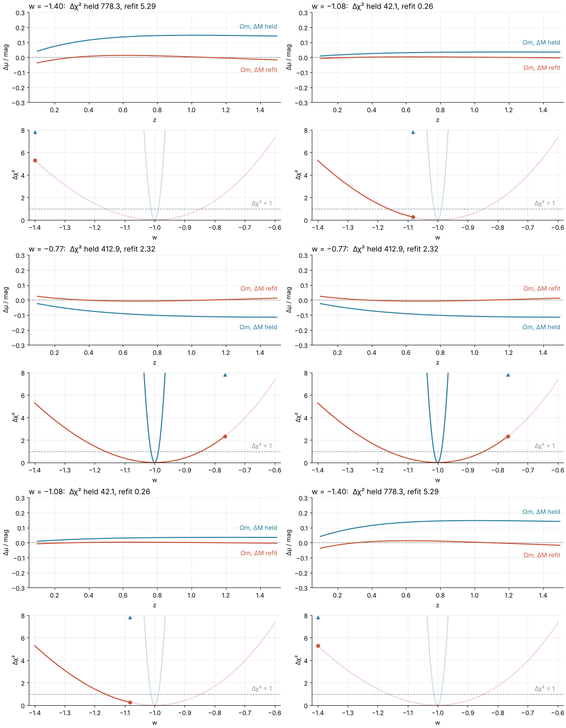
Held, the score at w = −0.9 is Δχ² = 69. Refit, it is 0.40: a lower Ωm and a slightly larger offset bend the curve back onto the fiducial one to within 0.010 mag, a fifteenth of an error bar. Even at w = −0.7 the refit keeps Δχ² under 4. Sweep w through −1 and trace both scores:

w sweeps from −1.4 to −0.6 and back. Top: the shift of the model from the fiducial survey with Ωm and ΔM held, which grows to +0.15 mag at w = −1.4 and −0.22 mag at w = −0.6, and with them refit, which stays near zero. Bottom: Δχ² against w; the held curve is a narrow spike, the refit one a wide parabola that crosses the dashed Δχ² = 1 near −1.17 and −0.84.

Show code

"""w sweep: how fast chi^2 rises as w moves away from -1, with Omega_m and Delta M held or refit.

Renders ../../assets/w-sweep.gif from the survey of the tutorial (same constants, same seed).
Run it from any directory:

    python scene.py
"""
from pathlib import Path

import numpy as np
import matplotlib.pyplot as plt
from matplotlib.animation import FuncAnimation, PillowWriter
from scipy.integrate import quad
from scipy.interpolate import CubicSpline
from scipy.optimize import least_squares

OUT = Path(__file__).resolve().parents[2] / "assets" / "w-sweep.gif"
INK, ACCENT, SECOND, MUTED = "#1f2a44", "#c8553d", "#2a7f9e", "#8a8f98"
plt.rcParams.update({"axes.spines.top": False, "axes.spines.right": False,
                     "axes.grid": True, "grid.alpha": 0.25, "font.size": 11})

# ---- data: the noise-free survey of the tutorial
C_KMS, H0, SIGMA, N = 299_792.458, 70.0, 0.15, 1000
rng = np.random.default_rng(244)
z = np.sort(rng.uniform(0.1, 1.5, N))
z_grid = np.linspace(0, 1.5, 151)


def mu(Om, w, dM):
    E = lambda x: np.sqrt(Om * (1 + x) ** 3 + (1 - Om) * (1 + x) ** (3 * (1 + w)))
    pieces = [quad(lambda x: 1 / E(x), a, b, epsabs=0, epsrel=1e-12)[0]
              for a, b in zip(z_grid[:-1], z_grid[1:])]
    D = CubicSpline(z_grid, np.concatenate([[0.0], np.cumsum(pieces)]))(z)
    return 5 * np.log10((1 + z) * C_KMS / H0 * D) + 25 + dM


mu_fid = mu(0.3, -1.0, 0.0)


def held_and_refit(w):
    """Residual curves and Delta chi^2 with Omega_m, Delta M held, and with them refit."""
    held = mu(0.3, w, 0.0) - mu_fid
    r = least_squares(lambda q: (mu(q[0], w, q[1]) - mu_fid) / SIGMA, [0.3, 0.0],
                      bounds=([0.01, -1], [1, 1]))
    return held, r.fun * SIGMA, np.sum((held / SIGMA) ** 2), 2 * r.cost


# w runs from -1.4 to -0.6 and back, with a short hold at each end, so the loop has no seam.
sweep = np.linspace(-1.4, -0.6, 49)
frames = np.concatenate([sweep, [sweep[-1]] * 4, sweep[-2:0:-1], [sweep[0]] * 4])
results = [held_and_refit(w) for w in sweep]
chi2_refit = np.array([r[3] for r in results])
w_fine = np.linspace(-1.1, -0.9, 201)                                # the held parabola is narrow
chi2_held_fine = np.array([np.sum(((mu(0.3, w, 0.0) - mu_fid) / SIGMA) ** 2) for w in w_fine])

# ---- figure, drawn once
fig, (ax1, ax2) = plt.subplots(2, 1, figsize=(7, 6.0), dpi=80, layout="constrained")
ax1.axhline(0, color=MUTED, lw=1, ls="--")
(held_line,) = ax1.plot([], [], color=SECOND, lw=1.8)
(refit_line,) = ax1.plot([], [], color=ACCENT, lw=1.8)
held_label = ax1.text(1.5, 0, "Ωm, ΔM held", color=SECOND, ha="right")
refit_label = ax1.text(1.5, 0, "Ωm, ΔM refit", color=ACCENT, ha="right")
ax1.set(xlim=(0.05, 1.52), ylim=(-0.3, 0.3), xlabel="z", ylabel="Δμ / mag")
ax2.axhline(1, color=MUTED, lw=1, ls="--")
ax2.text(-0.61, 1.15, "Δχ² = 1", color=MUTED, ha="right", va="bottom")
ax2.plot(w_fine, chi2_held_fine, color=SECOND, lw=1.8, alpha=0.25)
ax2.plot(sweep, chi2_refit, color=ACCENT, lw=1.8, alpha=0.25)
(held_trace,) = ax2.plot([], [], color=SECOND, lw=1.8)
(refit_trace,) = ax2.plot([], [], color=ACCENT, lw=1.8)
(held_dot,) = ax2.plot([], [], "o", color=SECOND, ms=6)
(refit_dot,) = ax2.plot([], [], "o", color=ACCENT, ms=6)
ax2.set(xlim=(-1.42, -0.58), ylim=(0, 8), xlabel="w", ylabel="Δχ²")
title1 = ax1.set_title("", loc="left")


# ---- one frame: a function of w alone
def update(i):
    w = frames[i]
    k = np.argmin(np.abs(sweep - w))
    held, refit, c_held, c_refit = results[k]
    held_line.set_data(z, held)
    refit_line.set_data(z, refit)
    # each label sits beside the end of its curve, the held one on the far side from zero
    side = 1 if held[-1] >= 0 else -1
    held_label.set_position((1.5, held[-1] + 0.04 * side))
    held_label.set_va("bottom" if side > 0 else "top")
    refit_label.set_position((1.5, refit[-1] - 0.04 * side))
    refit_label.set_va("top" if side > 0 else "bottom")
    upto = sweep <= w + 1e-9
    shown = w_fine <= w + 1e-9
    held_trace.set_data(w_fine[shown], chi2_held_fine[shown])
    refit_trace.set_data(sweep[upto], chi2_refit[upto])
    held_dot.set_data([w], [min(c_held, 7.8)])        # pinned to the top, as a triangle, once it leaves the plot
    held_dot.set_marker("o" if c_held < 7.8 else "^")
    refit_dot.set_data([w], [c_refit])
    title1.set_text(f"w = {w:+.2f}:  Δχ² held {c_held:.1f}, refit {c_refit:.2f}".replace("-", "−"))


# ---- render, and read back what was written
OUT.parent.mkdir(exist_ok=True)
FuncAnimation(fig, update, frames=len(frames)).save(OUT, writer=PillowWriter(fps=12))
plt.close(fig)
print(f"{OUT.name}: {len(frames)} frames at 12 fps, {len(frames) / 12:.1f} s, "
      f"{OUT.stat().st_size / 1024:,.0f} kB")

Which rise counts as one standard deviation? Least squares showed that the probability of the data under a model is proportional to \(e^{-\chi^2/2}\). A rise of Δχ² = 1 makes the data \(e^{1/2} = 1.65\) times less probable than at the bottom, and a bell curve in w, \(e^{-(w+1)^2/2\sigma^2}\), falls by exactly that factor at one σ from its center. So the error on w sits where the score has risen by one:

Show code

held_dchi2 = lambda w: chi2(mu(z, 0.3, w, 0.0)) - 1
refit_dchi2 = lambda w: refit(w)[1] - 1
for name, f in [("held", held_dchi2), ("refit", refit_dchi2)]:
    w_minus, w_plus = brentq(f, -1.5, -1.0001), brentq(f, -0.9999, -0.6)
    print(f"{name:5s}  Δχ² = 1 at w = {w_minus:+.4f} and {w_plus:+.4f}, "
          f"half-width {(w_plus - w_minus) / 2:.4f}")

held   Δχ² = 1 at w = -1.0125 and -0.9876, half-width 0.0125
refit  Δχ² = 1 at w = -1.1658 and -0.8446, half-width 0.1606

Held, Δχ² crosses 1 at w = −1 ± 0.0125. Refit, it crosses at −1.166 and −0.845, a half-width of 0.161 and already a little lopsided. The first number is called the conditional error: the error on w if Ωm and ΔM were known exactly. The second is the marginalized error: the error on w when Ωm and ΔM have to be measured from the same data. The word has a stricter meaning, which the formalization gives; for a score that rises like a parabola it agrees with the refit.

Why the error on w is thirteen times larger than it looks

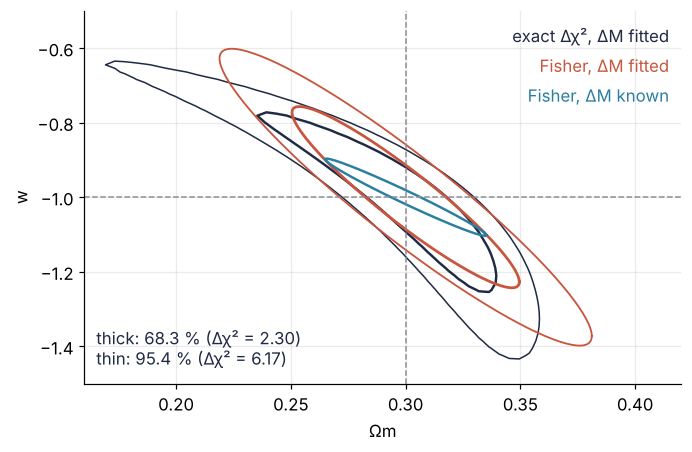
The refit hides a trade. Draw Δχ² over the whole (Ωm, w) plane and the trade becomes a valley. ΔM is refit at each point for free: μ depends on it only as an added constant, so the best offset is the mean residual. For one parameter, Δχ² = 1 and 4 enclose 68.3 % and 95.4 % of surveys, one and two σ of a bell curve. For two parameters at once, the regions that hold the same shares reach Δχ² = 2.30 and 6.17, because two directions share the scatter. Both are quantiles of the chi-square distribution with two degrees of freedom, the family Least squares used for the χ² at the bottom of a fit.

On top of the exact contours the figure draws the forecast: ellipses from the Fisher matrix, which the formalization below defines. Each ellipse is the bowl that matches Δχ² at the bottom of the valley, computed from the slopes of μ at the fiducial values alone. One pair of ellipses has ΔM fitted, like the exact contours, and a narrower one has ΔM known. The table under the figure lists the error on w with Ωm and ΔM each held or fitted.

Show code

def jacobian(z, p, h=1e-4):
    """d mu / d parameter at p by central differences, one column per parameter."""
    J = np.empty((z.size, p.size))
    for i in range(p.size):
        dp = np.zeros(p.size)
        dp[i] = h
        J[:, i] = (mu(z, *(p + dp)) - mu(z, *(p - dp))) / (2 * h)
    return J


J = jacobian(z, p_fid)
F = J.T @ J / SIGMA**2
cov = np.linalg.inv(F)
cov_dM_known = np.linalg.inv(F[:2, :2])


def ellipse(cov2, level, n=200):
    """Points of the Fisher ellipse Delta chi^2 = level around the fiducial (Omega_m, w)."""
    t = np.linspace(0, 2 * np.pi, n)
    L = np.linalg.cholesky(cov2)
    return p_fid[:2, None] + np.sqrt(level) * L @ np.vstack([np.cos(t), np.sin(t)])


# Exact Delta chi^2 with Delta M refit at each point: mu is linear in Delta M,
# so the best offset is the mean residual and the rest is the scatter about it.
Om_axis = np.linspace(0.16, 0.42, 60)
w_axis = np.linspace(-1.6, -0.45, 60)
dchi2 = np.empty((w_axis.size, Om_axis.size))
for i, w in enumerate(w_axis):
    for j, Om in enumerate(Om_axis):
        r = mu(z, Om, w, 0.0) - mu_fid
        dchi2[i, j] = np.sum((r - r.mean()) ** 2) / SIGMA**2

fig, ax = plt.subplots(figsize=(7, 4.4))
ax.contour(Om_axis, w_axis, dchi2, levels=[2.30, 6.17], colors=INK, linewidths=[1.6, 1.0])
for level, lw in [(2.30, 1.8), (6.17, 1.2)]:
    ax.plot(*ellipse(cov[:2, :2], level), color=ACCENT, lw=lw)
ax.plot(*ellipse(cov_dM_known, 2.30), color=SECOND, lw=1.6)
ax.axvline(0.3, color=MUTED, lw=1, ls="--")
ax.axhline(-1.0, color=MUTED, lw=1, ls="--")
for y, label, color in [(0.96, "exact Δχ², ΔM fitted", INK), (0.88, "Fisher, ΔM fitted", ACCENT),
                        (0.80, "Fisher, ΔM known", SECOND)]:
    ax.text(0.98, y, label, color=color, transform=ax.transAxes, ha="right", va="top")
ax.text(0.02, 0.04, "thick: 68.3 % (Δχ² = 2.30)\nthin: 95.4 % (Δχ² = 6.17)", color=INK,
        transform=ax.transAxes, ha="left", va="bottom")
ax.set(xlabel="Ωm", ylabel="w", xlim=(Om_axis[0], Om_axis[-1]), ylim=(-1.5, -0.5))
plt.show()


def sigma_w(F, free):
    """sigma(w) with the parameters in `free` marginalized and the others held."""
    keep = [1] + list(free)              # w first
    return np.sqrt(np.linalg.inv(F[np.ix_(keep, keep)])[0, 0])


print("σ(w)              ΔM held    ΔM fitted")
print(f"  Ωm held         {sigma_w(F, []):7.4f}    {sigma_w(F, [2]):7.4f}")
print(f"  Ωm fitted       {sigma_w(F, [0]):7.4f}    {sigma_w(F, [0, 2]):7.4f}")

The (Ωm, w) plane with the exact Δχ² contours at 2.30 and 6.17 (68.3 % and 95.4 %) and the Fisher ellipses at the same levels, ΔM fitted, all tilted from upper left to lower right. A narrow ellipse for ΔM known lies inside. At 95.4 % the exact contour bends into a banana toward low Ωm and high w.

σ(w)              ΔM held    ΔM fitted
  Ωm held          0.0125     0.0569
  Ωm fitted        0.0683     0.1603

The valley runs from the upper left to the lower right: a lower Ωm buys a less negative w, which is the refit at w = −0.9 seen from above. The 1σ errors are read off the ellipse at Δχ² = 1, which is the 68.3 % ellipse shrunk by \(\sqrt{2.30} = 1.52\). At each w, refitting Ωm and ΔM finds the lowest point of the valley, so the shadow of that ellipse on the w axis ends where the refit score of the previous section has risen by one: the marginalized error, 0.160. Its cut along the dashed line Ωm = 0.3 is the error with Ωm held and ΔM still fitted, 0.057. The narrow ellipse for ΔM known has a shadow of 0.068 and a cut of 0.0125. Every parameter you let go widens the ellipse, and the nuisance offset alone more than doubles σ(w). From 0.0125 with both held to 0.160 with both fitted is the factor of thirteen in the heading.

At 68.3 % the exact contour and the Fisher ellipse nearly coincide. At 95.4 % they part: the exact contour bends away toward low Ωm and high w into a banana, and the ellipse cannot follow, because an ellipse is all a quadratic approximation can draw.

The question

The idea: how fast the fit gets worse

Why the error on w is thirteen times larger than it looks

The second half of this tutorial needs a free account