Least squares: what a fit minimizes, and why the residuals are squared

The question

A temperature sensor is calibrated against a reference thermometer at eight temperatures, from −20 to 50 °C in steps of 10. Its reading should follow a straight line, reading = a + b·T, where the intercept a is the reading at 0 °C and the slope b is the sensitivity. The datasheet promises 500 mV and 10 mV/°C. Each reading has an error bar, 5 mV at −20 °C growing to 19 mV at 50 °C, because the reference bath is less stable when hot. Least squares is the rule nearly everyone uses to pick a line through such readings. Here are the eight, with three lines drawn by eye:

Show code

Copy

import itertools
import numpy as np
import matplotlib.pyplot as plt

plt.rcParams.update({
    "figure.figsize": (7, 3.6), "figure.dpi": 110,
    "axes.spines.top": False, "axes.spines.right": False,
    "axes.grid": True, "grid.alpha": 0.25,
    "font.size": 11, "lines.linewidth": 1.8,
})
INK, ACCENT, SECOND, MUTED = "#1f2a44", "#c8553d", "#2a7f9e", "#8a8f98"

# The readings are simulated from a sensor that is exactly nominal, so the answer can be checked.
A_NOM, B_NOM = 500.0, 10.0                     # datasheet: mV at 0 °C, mV/°C
T = np.arange(-20, 51, 10.0)                   # °C
sigma = 5 + 0.2 * (T + 20)                     # mV; the reference bath is less stable when hot
rng = np.random.default_rng(7)
y = A_NOM + B_NOM * T + sigma * rng.standard_normal(T.size)
guesses = {"A": (485.0, 10.5), "B": (515.0, 9.5), "C": (510.0, 10.0)}   # (a / mV, b / (mV/°C))

def deviation(a, b, T):
    """A line a + b T, measured from the datasheet line, in mV."""
    return a + b * T - (A_NOM + B_NOM * T)

dev = y - (A_NOM + B_NOM * T)
print("T / °C        " + " ".join(f"{t:6.0f}" for t in T))
print("reading / mV  " + " ".join(f"{v:6.1f}" for v in y))
print("deviation / mV" + " ".join(f"{v:6.1f}" for v in dev))
print("σ / mV        " + " ".join(f"{s:6.1f}" for s in sigma))
for name, (a, b) in guesses.items():
    r = y - a - b * T
    print(f"guess {name}: misses {np.sum(np.abs(r) > sigma)} of {T.size} readings by more than their error bar")

T_line = np.array([-25.0, 55.0])
fig, (ax1, ax2) = plt.subplots(2, 1, figsize=(7, 5), sharex=True)
for ax, base in [(ax1, 0 * T), (ax2, A_NOM + B_NOM * T)]:
    base_line = 0 * T_line if ax is ax1 else A_NOM + B_NOM * T_line
    for name, (a, b) in guesses.items():
        ax.plot(T_line, a + b * T_line - base_line, color=SECOND, lw=1.2)
    ax.errorbar(T, y - base, sigma, fmt="o", ms=4, capsize=2, lw=1, color=INK, zorder=3)
ax2.axhline(0, color=MUTED, lw=1, ls="--")
for name, (a, b) in guesses.items():
    ax2.text(-26, deviation(a, b, -25.0), name, color=SECOND, ha="right", va="center")
ax1.set(ylabel="reading / mV")
ax2.set(xlabel="T / °C", ylabel="deviation / mV", xlim=(-30, 55), ylim=(-45, 50))
plt.show()

T / °C           -20    -10      0     10     20     30     40     50
reading / mV   300.0  402.1  497.5  590.2  694.1  785.1  901.0 1025.5
deviation / mV   0.0    2.1   -2.5   -9.8   -5.9  -14.9    1.0   25.5
σ / mV           5.0    7.0    9.0   11.0   13.0   15.0   17.0   19.0
guess A: misses 3 of 8 readings by more than their error bar
guess B: misses 5 of 8 readings by more than their error bar
guess C: misses 6 of 8 readings by more than their error bar

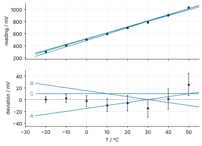
Two things are obvious. The readings lie on a line, and at full scale all three guesses lie on it too: A (485 mV, 10.5 mV/°C), B (515 mV, 9.5 mV/°C), and C (510 mV, 10.0 mV/°C) are hard to tell apart on an axis that spans 900 mV. The bottom panel subtracts the datasheet line from everything, and there they part. A misses 3 of the 8 readings by more than their error bar, B misses 5, and C, whose slope is exactly the datasheet's, misses 6.

Less obvious: of all the lines you could draw, which one is best, and by what score? "Closest to the points" means nothing until it is a number, and that number has to decide what to do with a reading whose error bar is four times longer than another's.

The readings are simulated from a sensor that is exactly nominal, so every answer can be checked against 500 mV and 10 mV/°C. I picked seed 7 because its least certain reading, at 50 °C, lands 25.5 mV high, which shows the pull the error bars remove later. Every plot from here on uses the deviation view: a 25 mV miss is invisible on a 900 mV axis.

The idea: score a line by the squares of its misses

A residual is the vertical gap between a reading and a line, rᵢ = yᵢ − a − b·Tᵢ. Summing the residuals fails at once: misses above and below cancel, and a line can score zero while missing every reading. Squaring makes every miss count, so the score of a line is the sum of squared residuals,

in mV². Drawn literally, each residual is the side of a square, and S is the total area of the squares:

Show code

Copy

def sum_sq(a, b):
    """S(a, b): the plain sum of squared residuals of the line a + b T, in mV²."""
    return np.sum((y - a - b * T) ** 2)

def draw_squares(ax, a, b, color):
    """Each residual as a square of side |r| that looks square on screen."""
    fig_w, fig_h = ax.figure.get_size_inches()
    pos = ax.get_position()
    (x0, x1), (y0, y1) = ax.get_xlim(), ax.get_ylim()
    per_mv = ((x1 - x0) / (pos.width * fig_w)) / ((y1 - y0) / (pos.height * fig_h))   # °C per mV on screen
    line = deviation(a, b, T)
    for Ti, li, di in zip(T, line, dev):
        side = abs(di - li)
        ax.add_patch(plt.Rectangle((Ti, min(li, di)), side * per_mv, side, color=color, alpha=0.35, lw=0))
        ax.plot([Ti, Ti], [li, di], color=color, lw=1)

fig, axes = plt.subplots(3, 1, figsize=(7, 6.6), sharex=True)
for ax, (name, (a, b)) in zip(axes, guesses.items()):
    ax.set(xlim=(-25, 62), ylim=(-45, 45), ylabel="deviation / mV")
    ax.axhline(0, color=MUTED, lw=1, ls="--")
    ax.plot(T_line, deviation(a, b, T_line), color=SECOND, lw=1.2)
    draw_squares(ax, a, b, SECOND)                      # the squares belong to the guessed line
    ax.plot(T, dev, "o", ms=4, color=INK, zorder=3)
    ax.text(0.01, 0.95, f"{name}:  S = {sum_sq(a, b):,.0f} mV²", transform=ax.transAxes, va="top", color=SECOND)
axes[-1].set(xlabel="T / °C")
plt.show()

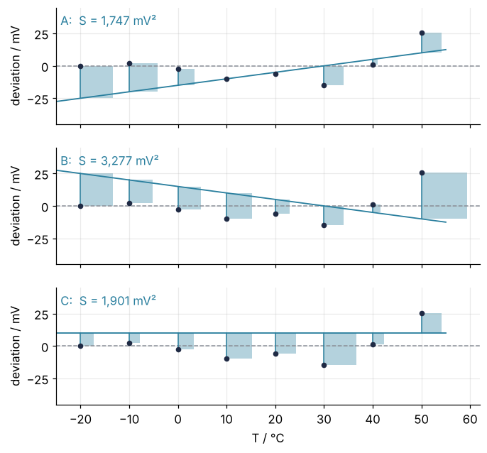
C has the datasheet's slope and looks like the best guess, yet A scores lower, 1,747 mV² against 1,901. C misses all eight readings, by 7.9 to 24.9 mV; A gets three within 4 mV. The score judges large misses harshly: one 20 mV miss costs as much as four 10 mV misses, and B, with 35.5 mV at 50 °C, scores 3,277 mV².

Now the step that turns least squares into a picture. The readings are fixed, so S depends on nothing but a and b. Every line is a point in a plane, slope on one axis and intercept on the other, and its score is a height above that point: a landscape, whose lowest point is the best line. Watch a line wander from A past B and C and come to rest, with its squares on the left and its point on the landscape on the right:

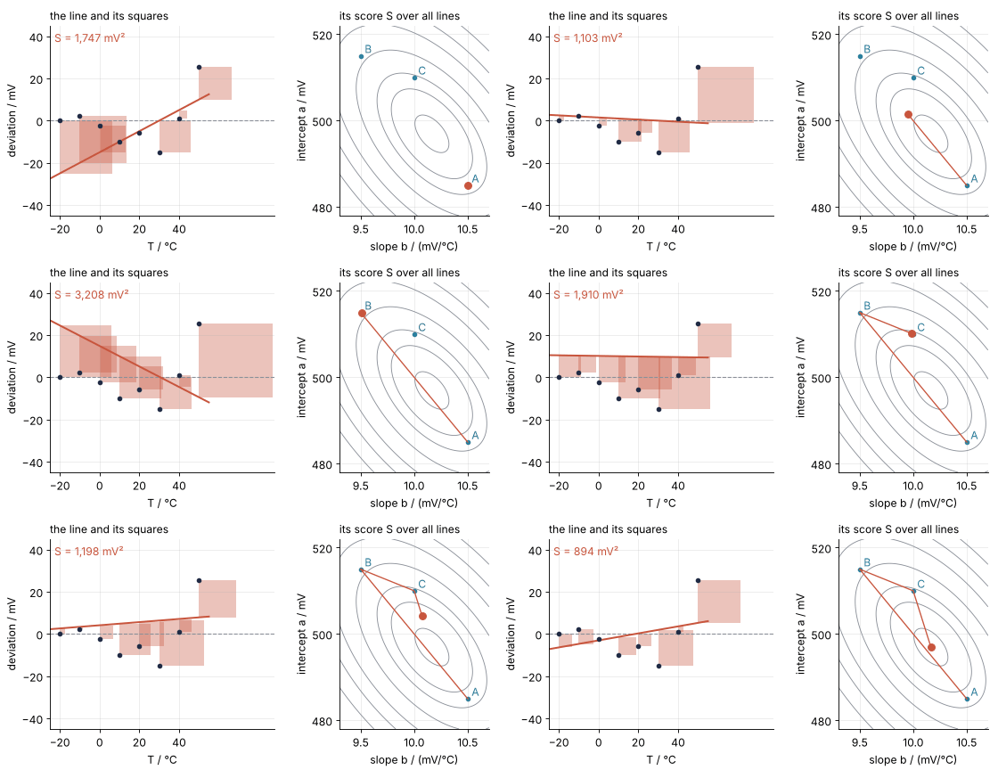
How I built this: each frame moves the line one step along a path from A to the bottom and redraws its squares and its trail with Matplotlib's FuncAnimation, the technique of Matplotlib animation with FuncAnimation; the source is animations/residual-squares/scene.py.

Here is the whole landscape as a contour map:

Show code

Copy

def fit(T, y, sigma):
    """The exact bottom of the bowl: least squares with rows divided by σ (Formalization shows what this solves)."""
    X = np.column_stack([np.ones_like(T), T])
    return np.linalg.lstsq(X / sigma[:, None], y / sigma, rcond=None)[0]

# Every line is a point (b, a); the score is evaluated on a grid of 301 × 301 lines at once.
a_grid = np.linspace(478, 522, 301)
b_grid = np.linspace(9.3, 10.7, 301)
B_mesh, A_mesh = np.meshgrid(b_grid, a_grid)
resid = y - A_mesh[..., None] - B_mesh[..., None] * T          # shape (301, 301, 8)
S_map = np.sum(resid ** 2, axis=-1)

a_u, b_u = fit(T, y, np.ones_like(T))
print(f"bottom of S: a = {a_u:.2f} mV, b = {b_u:.3f} mV/°C, S = {sum_sq(a_u, b_u):,.0f} mV²")

def mark_guesses(ax):
    for name, (a, b) in guesses.items():
        ax.plot(b, a, "o", ms=6, color=SECOND)
        ax.annotate(name, (b, a), xytext=(6, 4), textcoords="offset points", color=SECOND)

fig, ax = plt.subplots(figsize=(7, 4))
cs = ax.contour(B_mesh, A_mesh, S_map, levels=[1000, 1500, 2000, 3000, 4500, 6000, 8000], colors=MUTED, linewidths=1)
ax.clabel(cs, levels=[1000, 2000, 4500, 8000], fmt="%d mV²", fontsize=11,
          manual=[(10.05, 502), (10.45, 506), (9.75, 482), (10.55, 519)])     # one label per level, clear of the dots
mark_guesses(ax)
ax.plot(b_u, a_u, "o", ms=6, color=ACCENT)
ax.annotate(f"bottom, {sum_sq(a_u, b_u):,.0f} mV²", (b_u, a_u), xytext=(8, -12), textcoords="offset points", color=ACCENT,
            bbox=dict(fc="white", ec="none", pad=1))
ax.set(xlabel="slope b / (mV/°C)", ylabel="intercept a / mV")
plt.show()

bottom of S: a = 496.95 mV, b = 10.166 mV/°C, S = 894 mV²

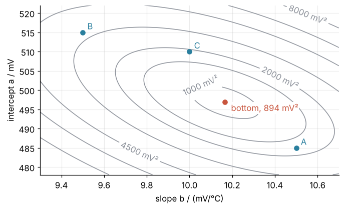
The landscape is a bowl with one bottom, and the guesses sit on its walls, A lowest and B highest, as their squares said. The bottom is the least-squares line, a = 496.95 mV and b = 10.166 mV/°C, with S = 894 mV², half of A's score.

Why squares and not absolute values

The sum of absolute values, Σ|rᵢ|, also makes every miss count, and it charges a 20 mV miss twice a 10 mV miss instead of four times. Its bottom has no formula, but a short argument finds it. Take a line that touches no reading and raise it by 1 mV. Every reading above the line gets 1 mV closer and every reading below gets 1 mV farther, so Σ|r| changes by the same amount for each millivolt, and lowering the line reverses the sign. One of the two directions does not raise the score, so move the line that way until it touches a reading. Then turn it about that reading: the same counting applies, and the line reaches a second reading without its score rising. A best line is always among the 28 lines through two readings, and the code scores all of them:

def sum_abs(a, b, y=y):
    return np.sum(np.abs(y - a - b * T))

def best_abs_lines(y):
    """All 28 lines through two readings, ranked by the sum of absolute residuals."""
    lines = []
    for i, j in itertools.combinations(range(T.size), 2):
        b = (y[j] - y[i]) / (T[j] - T[i])
        a = y[i] - b * T[i]
        lines.append((sum_abs(a, b, y), a, b, T[i], T[j]))
    return sorted(lines)

ranked = best_abs_lines(y)
tied = [line for line in ranked if line[0] - ranked[0][0] < 1e-9]
for score, a, b, Ti, Tj in tied:
    print(f"through the readings at {Ti:4.0f} and {Tj:3.0f} °C:  a = {a:.2f} mV, b = {b:.3f} mV/°C, Σ|r| = {score:.2f} mV")

through the readings at  -20 and   0 °C:  a = 497.53 mV, b = 9.876 mV/°C, Σ|r| = 61.63 mV
through the readings at  -20 and  40 °C:  a = 500.34 mV, b = 10.017 mV/°C, Σ|r| = 61.63 mV
through the readings at    0 and  40 °C:  a = 497.53 mV, b = 10.087 mV/°C, Σ|r| = 61.63 mV

Three lines tie. Here are both landscapes over the same plane:

Show code

Copy

abs_map = np.sum(np.abs(resid), axis=-1)
corners = np.array([(b, a) for _, a, b, _, _ in tied])

fig, (ax1, ax2) = plt.subplots(2, 1, figsize=(7, 6.4), sharex=True)
ax1.contour(B_mesh, A_mesh, S_map, levels=[1000, 1500, 2000, 3000, 4500, 6000, 8000], colors=MUTED, linewidths=1)
ax1.plot(b_u, a_u, "o", ms=6, color=ACCENT)
ax1.text(0.01, 0.95, "sum of squares", transform=ax1.transAxes, va="top", bbox=dict(fc="white", ec="none", pad=1))
ax2.contour(B_mesh, A_mesh, abs_map, levels=[64, 70, 80, 95, 115, 140, 170], colors=MUTED, linewidths=1)
ax2.fill(corners[:, 0], corners[:, 1], color=ACCENT, alpha=0.35, lw=0)
ax2.plot(corners[:, 0], corners[:, 1], "o", ms=4, color=ACCENT)
ax2.text(0.01, 0.95, "sum of absolute values", transform=ax2.transAxes, va="top", bbox=dict(fc="white", ec="none", pad=1))
ax1.set(ylabel="intercept a / mV")
ax2.set(xlabel="slope b / (mV/°C)", ylabel="intercept a / mV")
plt.show()

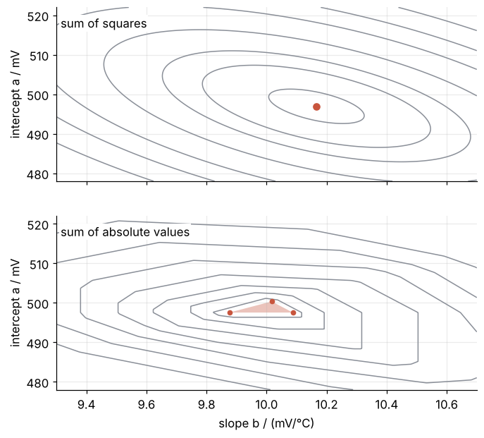
The squares give a smooth, round bowl. The absolute values give a landscape of flat facets meeting in creases, and here its bottom is a flat triangle: every line inside it scores the same 61.63 mV, with slopes from 9.876 to 10.087 mV/°C, so "the best line" has no single answer. Its corners are the three tied lines, through the readings at −20 and 0 °C, at −20 and 40 °C, and at 0 and 40 °C.

Squares have a price. Push the 30 °C reading up by 80 mV, as a loose connector might, and then by 160 mV:

print("30 °C reading     least squares     absolute values")
for push in [0, 80, 160]:
    y_out = y.copy()
    y_out[T == 30] += push
    _, b_ls = fit(T, y_out, np.ones_like(T))
    ranked_out = best_abs_lines(y_out)
    tied_out = [line for line in ranked_out if line[0] - ranked_out[0][0] < 1e-9]
    slopes = sorted(line[2] for line in tied_out)
    l1 = f"{slopes[0]:.3f}" if len(slopes) == 1 else f"tie, {slopes[0]:.3f} to {slopes[-1]:.3f}"
    print(f"  + {push:3d} mV        {b_ls:6.3f} mV/°C      {l1} mV/°C")

30 °C reading     least squares     absolute values
  +   0 mV        10.166 mV/°C      tie, 9.876 to 10.087 mV/°C
  +  80 mV        10.452 mV/°C      10.017 mV/°C
  + 160 mV        10.738 mV/°C      10.017 mV/°C

The least-squares slope follows the bad reading, from 10.17 to 10.45 and then 10.74 mV/°C. The absolute-value fit settles on one corner of the triangle it already had, the line through the −20 and 40 °C readings at 10.017 mV/°C, and stays on that same line at +160 mV. The outlier only breaks the tie; it does not move the answer out of the set that was best without it. Squares cannot ignore a reading, however wild. Formalization gives the reason they are used anyway.

Dividing by the error bar

The plain sum S treats every reading alike. An error bar σ is one standard deviation of a reading's Gaussian scatter, the promise that The standard error of the mean explains. A miss of 19 mV at 50 °C is one error bar there, the kind of miss the reference bath produces routinely, while the same 19 mV at −20 °C is nearly four error bars, which Gaussian scatter produces about once in 7,000 readings. Measure each residual in units of its own error bar, rᵢ/σᵢ, and square that. The score becomes

called chi-square, a pure number. Two things change. First, precise readings now pull harder than imprecise ones:

Show code

Copy

_, b_unweighted = fit(T, y, np.ones_like(T))
a_w, b_w = fit(T, y, sigma)
print(f"slope, every reading counted alike:     {b_unweighted:.2f} mV/°C")
print(f"slope, each residual divided by its σ:  {b_w:.2f} mV/°C   (truth {B_NOM:.2f})")

fig, ax = plt.subplots()
ax.axhline(0, color=MUTED, lw=1, ls="--")
ax.errorbar(T, dev, sigma, fmt="o", ms=4, capsize=2, lw=1, color=INK, zorder=3)
ax.plot(T_line, deviation(a_u, b_u, T_line), color=SECOND)
ax.plot(T_line, deviation(a_w, b_w, T_line), color=ACCENT)
ax.text(55.5, deviation(a_u, b_u, 55) + 1, f"unweighted\n{b_unweighted:.2f} mV/°C", color=SECOND, va="bottom")
ax.text(55.5, deviation(a_w, b_w, 55) - 1, f"weighted\n{b_w:.2f} mV/°C", color=ACCENT, va="top")
ax.set(xlabel="T / °C", ylabel="deviation / mV", xlim=(-25, 72), ylim=(-40, 50))
plt.show()

slope, every reading counted alike:     10.17 mV/°C
slope, each residual divided by its σ:  9.98 mV/°C   (truth 10.00)

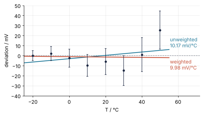
Unweighted, the 50 °C reading, 25.5 mV high, drags the slope to 10.17 mV/°C. Weighted, its long error bar lets it go, and the slope is 9.98 mV/°C against the true 10.00. Whenever your readings come with error bars, weight by them. An unweighted fit throws away what you know about your instrument.

Second, the score gets a scale. The bottom of the plain sum, 894 mV², changes with the units: the same fit scores 0.000894 V², and neither number says whether the fit is good. The bottom of χ² is 3.84 whether you work in millivolts or in volts, and a pure number can be compared with the number of readings.

Formalization

The least-squares fit is the pair a, b that minimizes

with Tᵢ, yᵢ, and σᵢ the temperature, reading, and error bar of reading i, and N = 8. With all σᵢ equal it is S divided by σ², with the same bottom.

Where the square and the σ come from. Suppose each reading scatters about the true line by a Gaussian of width σᵢ. The probability density of these readings under a given line is then proportional to \(\prod_i e^{-r_i^2/2\sigma_i^2} = e^{-\chi^2/2}\), so the line with the smallest χ² makes the observed readings most probable.

def chi2(a, b):
    return np.sum(((y - a - b * T) / sigma) ** 2)

N, n_par = T.size, 2
chi2_min = chi2(a_w, b_w)
for name, (a, b) in guesses.items():
    print(f"guess {name}:   χ² = {chi2(a, b):6.2f}")
print(f"the fit:   χ² = {chi2_min:6.2f}")
print(f"the readings are e^((χ²_C − χ²_min)/2) = {np.exp((chi2(*guesses['C']) - chi2_min) / 2):.0f} times "
      f"more probable under the fit than under C")

guess A:   χ² =  38.62
guess B:   χ² =  43.84
guess C:   χ² =  15.62
the fit:   χ² =   3.84
the readings are e^((χ²_C − χ²_min)/2) = 361 times more probable under the fit than under C

Guess C has χ² = 15.62 against the bottom's 3.84, so these readings are \(e^{(15.62 - 3.84)/2} = 361\) times more probable under the fitted line than under C. Squaring and dividing by σ are not matters of taste: Gaussian errors demand both.

One answer from linear algebra. At the bottom of the bowl the ground is flat in both directions, \(\partial\chi^2/\partial a = 0\) and \(\partial\chi^2/\partial b = 0\). χ² is quadratic in a and b, so its derivatives are linear in them, and the two conditions are two linear equations, the normal equations. With the weights wᵢ = 1/σᵢ² they read

with every sum over the eight readings:

w = 1 / sigma**2
# the normal equations, from the written-out weighted sums
lhs = np.array([[np.sum(w),     np.sum(w * T)],
                [np.sum(w * T), np.sum(w * T**2)]])
rhs = np.array([np.sum(w * y), np.sum(w * T * y)])
a_ne, b_ne = np.linalg.solve(lhs, rhs)
print(f"a = {a_ne:.2f} mV,  b = {b_ne:.3f} mV/°C")

a = 498.95 mV,  b = 9.982 mV/°C

The solve gives a = 498.95 mV and b = 9.982 mV/°C with no starting value and no search, as it does for any model linear in its parameters. In matrix form the system is \(X^\mathsf{T} W X\, p = X^\mathsf{T} W y\), with X the design matrix (a column of ones next to the column of the Tᵢ), W the diagonal matrix of the wᵢ, and p = (a, b). A model nonlinear in its parameters gives a bowl that is not quadratic, and curve_fit has to walk down to its bottom from a starting guess.

The minimum says whether the error bars are right. If the line is right and the error bars are honest, each term of χ² is about 1 on average. But the fit bends the line toward the readings, and each of the m = 2 fitted parameters uses up one reading's worth of scatter, so χ² at the bottom averages N − m = 6. N − m is called the degrees of freedom, dof, and χ²/dof averages 1. Ten thousand simulated calibrations show it:

Show code

Copy

# 10,000 calibrations of a nominal sensor with honest error bars, each refitted
sim = np.random.default_rng(2026)
X = np.column_stack([np.ones_like(T), T])
Y = (A_NOM + B_NOM * T) + sigma * sim.standard_normal((10_000, T.size))    # one calibration per row
P = np.linalg.lstsq(X / sigma[:, None], (Y / sigma).T, rcond=None)[0]       # all refits in one call
chi2_sim = np.sum(((Y - (X @ P).T) / sigma) ** 2, axis=1)
dof = N - n_par
lo, hi = np.percentile(chi2_sim / dof, [2.5, 97.5])
halved = 4 * chi2_min
print(f"mean χ² of 10,000 honest calibrations: {chi2_sim.mean():.2f}   (N − m = {dof})")
print(f"central 95 % of χ²/dof:                {lo:.2f} to {hi:.2f}")
print(f"this calibration:                      χ²/dof = {chi2_min / dof:.2f}")
print(f"with error bars stated at half size:   χ²/dof = {halved / dof:.2f}, "
      f"reached by {100 * np.mean(chi2_sim >= halved):.1f} % of honest calibrations")
print(f"scatter of the refits:                 a ± {P[0].std():.1f} mV,  b ± {P[1].std():.2f} mV/°C")

fig, ax = plt.subplots()
ax.axvspan(lo, hi, color=MUTED, alpha=0.15, lw=0)
counts, _, _ = ax.hist(chi2_sim / dof, bins=np.arange(0, 4.01, 0.08), color=MUTED, alpha=0.8, lw=0)
ax.axvline(chi2_min / dof, color=ACCENT, lw=1.8)
ax.axvline(halved / dof, color=SECOND, lw=1.2, ls="--")
ax.text(chi2_min / dof + 0.04, 0.93, f"this fit {chi2_min / dof:.2f}", transform=ax.get_xaxis_transform(), color=ACCENT, va="top")
ax.text(halved / dof + 0.04, 0.93, f"error bars halved {halved / dof:.2f}", transform=ax.get_xaxis_transform(), color=SECOND, va="top")
ax.text(hi - 0.04, 0.6, f"central 95 %\n{lo:.2f} to {hi:.2f}", transform=ax.get_xaxis_transform(), color=INK, ha="right")
ax.set(xlabel="χ² / dof", ylabel="calibrations", xlim=(0, 4), ylim=(0, 1.35 * counts.max()))
plt.show()

mean χ² of 10,000 honest calibrations: 5.99   (N − m = 6)
central 95 % of χ²/dof:                0.20 to 2.40
this calibration:                      χ²/dof = 0.64
with error bars stated at half size:   χ²/dof = 2.56, reached by 1.7 % of honest calibrations
scatter of the refits:                 a ± 3.3 mV,  b ± 0.17 mV/°C

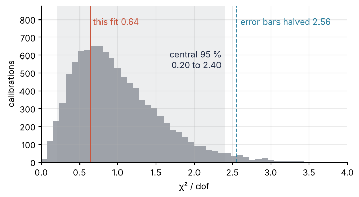
The mean χ² is 5.99, and the central 95 % of χ²/dof lies between 0.20 and 2.40. This calibration's 0.64 is unremarkable. With the error bars stated at half their size, χ² would be four times larger, χ²/dof = 2.56, beyond the band and reached by only 1.7 % of honest calibrations. Read the value this way: near 1, fine; far above, the model is wrong or the error bars are too small; far below, the error bars are too large.

How wide "near 1" is depends only on the degrees of freedom. With Gaussian errors and a model linear in its parameters, χ² at the bottom follows the chi-square distribution for N − m degrees of freedom, with mean N − m and standard deviation √(2(N − m)). Divided by the dof, that is a mean of 1 and a spread of √(2/dof). The function below checks it by fitting a polynomial of n_params coefficients to n_points honest readings at evenly spaced x with σ = 1, sharing only N and m with the calibration:

def chi2_band(n_points, n_params, draws=10_000):
    """Central 95 % of χ²/dof for a linear fit of n_params coefficients to n_points honest readings."""
    gen = np.random.default_rng(2026)
    x = np.linspace(-1, 1, n_points)
    X_poly = np.vander(x, n_params, increasing=True)
    E = gen.standard_normal((n_points, draws))            # σ = 1, the truth is zero
    coef = np.linalg.lstsq(X_poly, E, rcond=None)[0]
    chi2_draws = np.sum((E - X_poly @ coef) ** 2, axis=0)
    return np.percentile(chi2_draws / (n_points - n_params), [2.5, 97.5])

print(" N   m   dof   central 95 % of χ²/dof   1 ± 2√(2/dof)")
for n_points, n_params in [(8, 2), (15, 3), (52, 2)]:
    d = n_points - n_params
    lo_b, hi_b = chi2_band(n_points, n_params)
    print(f"{n_points:2d}  {n_params:2d}  {d:4d}   {lo_b:.2f} to {hi_b:.2f}             "
          f"{1 - 2 * np.sqrt(2 / d):5.2f} to {1 + 2 * np.sqrt(2 / d):.2f}")

 N   m   dof   central 95 % of χ²/dof   1 ± 2√(2/dof)
 8   2     6   0.20 to 2.42             -0.15 to 2.15
15   3    12   0.36 to 1.93              0.18 to 1.82
52   2    50   0.65 to 1.43              0.60 to 1.40

Eight readings and a line give 0.20 to 2.42, the calibration's band to within the simulation's scatter. From about 50 dof on, the distribution is close to a Gaussian, and the band is its mean ± two standard deviations, 1 ± 2√(2/dof), to within 0.05. Below that the band is lopsided; at 6 dof the Gaussian rule goes negative. For your own fit, scipy.stats.chi2.ppf([0.025, 0.975], dof) / dof returns the band: ppf takes a fraction q and the degrees of freedom and returns the χ² that a fraction q of honest fits stay below.

The ± of a fit. The refits of the simulation scatter by 3.3 mV in a and 0.17 mV/°C in b, and that is what 498.95 ± 3.3 mV means: one standard deviation of the fitted value over repeated calibrations.

See it in code

np.linalg.lstsq minimizes the plain sum of squares of a linear system, which is χ² once every row of X and every reading is divided by its σ. np.polyfit fits a polynomial and takes weights as an argument. Both, against the normal equations:

Show code

Copy

p, *_ = np.linalg.lstsq(X / sigma[:, None], y / sigma, rcond=None)    # rows divided by σ: weighted least squares
print(f"lstsq against the normal equations: largest difference {np.max(np.abs(p - [a_ne, b_ne])):.1e}")
b_pf, a_pf = np.polyfit(T, y, 1, w=1 / sigma)                          # polyfit wants 1/σ, not 1/σ²
print(f"polyfit, w = 1/σ:   largest difference {max(abs(a_pf - a_ne), abs(b_pf - b_ne)):.1e}")
b_wrong, _ = np.polyfit(T, y, 1, w=1 / sigma**2)
print(f"polyfit, w = 1/σ²:  b = {b_wrong:.2f} mV/°C")

chi2_map = np.sum((resid / sigma) ** 2, axis=-1)
fig, (ax1, ax2) = plt.subplots(2, 1, figsize=(7, 6), height_ratios=[1.4, 1])
ax1.contour(B_mesh, A_mesh, chi2_map, levels=[8, 12, 20, 30, 45, 60, 80], colors=MUTED, linewidths=1)   # inner oval wide enough for the label
mark_guesses(ax1)
ax1.plot(b_ne, a_ne, "o", ms=6, color=ACCENT)
ax1.annotate(f"χ² = {chi2_min:.2f}, {dof} dof", (b_ne, a_ne), xytext=(8, -14), textcoords="offset points", color=ACCENT,
             bbox=dict(fc="white", ec="none", pad=2))
ax1.set(xlabel="slope b / (mV/°C)", ylabel="intercept a / mV")
r_norm = (y - a_ne - b_ne * T) / sigma
ax2.axhline(0, color=MUTED, lw=1)
for level in [-1, 1]:
    ax2.axhline(level, color=MUTED, lw=1, ls="--")
ax2.vlines(T, 0, r_norm, color=ACCENT, lw=2)
ax2.plot(T, r_norm, "o", ms=6, color=ACCENT)
ax2.set(xlabel="T / °C", ylabel="residual / σ", ylim=(-2.2, 2.2))
fig.tight_layout()
plt.show()

lstsq against the normal equations: largest difference 1.1e-13
polyfit, w = 1/σ:   largest difference 5.7e-14
polyfit, w = 1/σ²:  b = 9.91 mV/°C

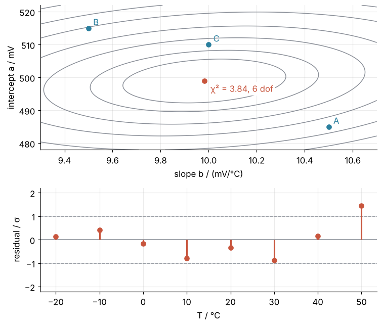
lstsq agrees with the normal equations to 1.1e-13 and polyfit to 5.7e-14, which is round-off. The polyfit documentation says its weight multiplies the residual before squaring, so for error bars it wants 1/σ. Hand it 1/σ², the usual inverse-variance weight, and every squared residual is weighted by 1/σ⁴: the slope comes out 9.91 mV/°C instead of 9.98, without a warning. Against the truth, 500 mV and 10.00 mV/°C both lie within one standard deviation of the fit, 498.95 ± 3.3 mV and 9.982 ± 0.17 mV/°C. Below the bowl are the eight residuals in units of their error bars, and their squares add up to the 3.84 at its bottom.

Where it shows up

• Engineering and physics: calibration lines. The gain and offset of a strain gauge or a load cell come from a weighted straight-line fit of its readings against a reference, exactly as here. χ²/dof tells you whether the stated uncertainty of the reference holds up.
• Chemistry: Beer-Lambert calibration. The absorbance of a set of standards against their concentration is a line whose slope is the molar absorption coefficient times the path length. The concentration of an unknown sample is read off the fitted line.
• Biochemistry and pharmacology: rate curves. Michaelis-Menten rates and dose-response curves are fitted by minimizing the same χ². Their models are nonlinear in the parameters, the case that curve_fit from the ground up and Fit a curve to data with error bars and draw a confidence band take up.
• Oceanography and signal processing: tides. Harmonic analysis fits sines and cosines of the known tidal frequencies to a sea-level record, and with the frequencies fixed the model is linear in its amplitudes. That fit separates the lunar and solar twice-daily tides from one week of data, where the spectrum in The Fourier transform shows a single merged bump.
• Biology and the social sciences: regression. Ordinary least squares, the linear regression that statistics packages run by default, is the unweighted case, every σ equal. Its bowl is the plain sum of squares S, the bowl the animation above runs down.
• Geodesy and navigation: positioning. A GPS receiver that sees more satellites than its four unknowns, three coordinates and its clock offset, takes its position as the least-squares solution of the range equations. Those equations are nonlinear, so the receiver linearizes them about its current estimate and solves the linear problem a few times over.

In every case the answer is the bottom of a bowl over the parameters, and the height of that bottom says whether the error bars were honest.

Further reading

• numpy.linalg.lstsq and numpy.polyfit, the second for its convention on w.
• John R. Taylor, An Introduction to Error Analysis (2nd ed., University Science Books, 1997), the chapters on least-squares fitting and on the chi-squared test.
• Press, Teukolsky, Vetterling, and Flannery, Numerical Recipes, the chapter "Modeling of Data", for weighted fits and χ² with the numerics behind them.
• Related tutorials on this site: curve_fit from the ground up: the Michaelis-Menten constants of an enzyme, for models nonlinear in their parameters; Fit a curve to data with error bars and draw a confidence band; The standard error of the mean: why four times the data halves the error; Minimization with scipy.optimize.minimize: the shape of a seven-atom cluster, for walking downhill on a bowl that is not quadratic; Matplotlib animation with FuncAnimation: a probe sweep as a small GIF, how the animation was built; planned: the same tutorial in Julia.
• Download the notebook. It was executed with the library versions in the header.