Flame graphs from cProfile: see which call chain takes the time (Python)

The problem: a slow function three calls deep

In Profiling with cProfile and timeit, a script moves 2,000 random walkers through 2,000 steps in a box, and its cProfile table says that one function, msd, takes about nine tenths of the run. On the machine that built this page that run takes 2.5 to 5 s under the profiler, never quite the same twice. The table answers "which function" one row at a time, and you rebuild the call chain yourself: <module> calls simulate, which calls msd. A flame graph draws the same profile as nested bars: one bar per function, as wide as the time spent in it, the functions it called stacked on top, and the script at the bottom. In a larger program the slow function sits several calls deep under wrappers, its rows scattered down the table; in the graph it is the widest bar high up.

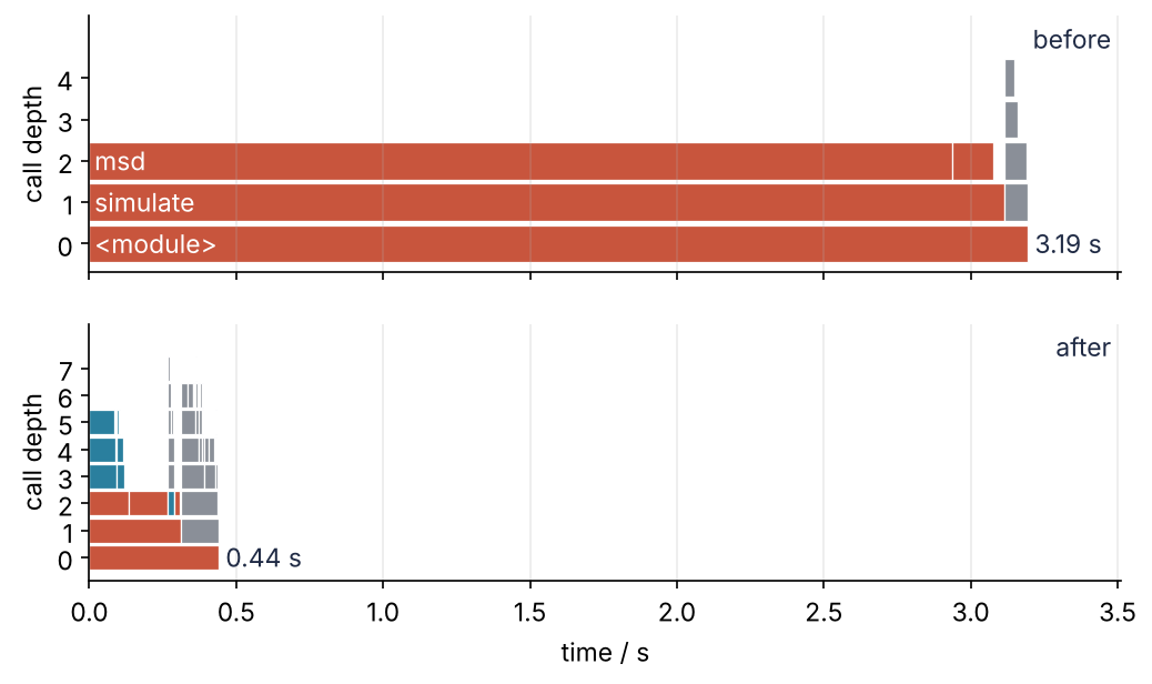
Flame graphs of the run before and after the fix, on one time axis in s. Red: functions of walkers.py; blue: NumPy; gray: Python itself. Before, the msd tower covers nearly the whole run of a few seconds; after, the whole run is a sliver of well under a second.

Here is the profile before the fix and after it, on one time axis. The msd tower that fills the first run is gone from the second, which is over in well under a second. The last step draws this figure from the two .prof files with nothing but pstats and Matplotlib; the steps before it work out where each bar goes.

Setup

The collapsed cell writes walkers.py, the script of the profiling tutorial, unchanged: open it to copy it, or skip it if you have the file. The block below it profiles the script twice in its own process, as it is and with --fast, the fix, and reuses the two .prof files when they exist. Your own script goes on the line marked # <- your script here.

Show code

%%writefile walkers.py
import sys
import numpy as np

def step(pos, size, rng):
    return pos + size * rng.standard_normal(pos.shape)

def reflect(pos, box):
    return box - np.abs(box - np.abs(pos))    # bounce off the walls at 0 and at box

def msd(pos, start):
    total = 0.0
    for i in range(len(pos)):                 # one walker at a time
        dx = pos[i, 0] - start[i, 0]
        dy = pos[i, 1] - start[i, 1]
        total += dx * dx + dy * dy
    return total / len(pos)
def msd_fast(pos, start):                     # the fix: the loop as one NumPy line
    return np.mean(np.sum((pos - start) ** 2, axis=1))

def simulate(msd=msd, n_walkers=2_000, n_steps=2_000, size=0.01, box=1.0, seed=1):
    rng = np.random.default_rng(seed)
    pos = start = box * rng.random((n_walkers, 2))
    curve = np.empty(n_steps)
    for t in range(n_steps):
        pos = reflect(step(pos, size, rng), box)
        curve[t] = msd(pos, start)            # the mean squared displacement after each step
    return curve

if __name__ == "__main__":  # true when run as a program, false on import
    simulate(msd_fast if "--fast" in sys.argv else msd)  # "python walkers.py --fast" runs the fix

Writing walkers.py

import os, pstats, subprocess, sys
import matplotlib.pyplot as plt

plt.rcParams.update({
    "figure.figsize": (7, 3.6), "figure.dpi": 110,
    "axes.spines.top": False, "axes.spines.right": False,
    "axes.grid": True, "grid.alpha": 0.25,
    "font.size": 11, "lines.linewidth": 1.8,
})
INK, ACCENT, SECOND, MUTED = "#1f2a44", "#c8553d", "#2a7f9e", "#8a8f98"

# ---- profile the script in its own process, as it is and with the fix
for name, flags in [("before", []), ("after", ["--fast"])]:
    if not os.path.exists(f"{name}.prof"):  # measures once for this page; drop this "if" in your copy
        subprocess.run([sys.executable, "-m", "cProfile", "-o", f"{name}.prof",
                        "walkers.py", *flags], check=True)     # <- your script here
for name in ["before", "after"]:
    print(f"{name}.prof: {pstats.Stats(f'{name}.prof').total_tt:.2f} s")

before.prof: 3.19 s
after.prof: 0.44 s

Step 1: Read who called whom from a cProfile file

pstats prints a profile as a table, but underneath it keeps a dict, Stats(...).stats, with one entry per function. The key is (file, line, name). The value holds the table's row, (primitive calls, calls, own time, cumulative time), and one thing the table does not print, the callers. They are a dict from each function that called this one to four numbers counted over that caller's calls alone, the edge between the two: the same four with the first two swapped, (calls, primitive calls, own time, cumulative time).

st = pstats.Stats("before.prof").stats
print(f"{len(st)} functions, {sum(f[0].endswith('walkers.py') for f in st)} of them in walkers.py")

msd = next(f for f in st if f[2] == "msd")
cc, nc, tt, ct, callers = st[msd]
print(f"{msd}: {nc} calls, own time {tt:.2f} s, cumulative {ct:.2f} s")
for f, (nc, cc, tt, ct) in callers.items():     # a caller's numbers start with all calls
    print(f"    called by {f[2]}: {nc} calls, {ct:.2f} s")

689 functions, 5 of them in walkers.py
('walkers.py', 10, 'msd'): 2000 calls, own time 2.93 s, cumulative 2.94 s
    called by simulate: 2000 calls, 2.94 s

Nearly 700 entries, five of them from walkers.py, and almost all the others come from importing NumPy and the parts of the standard library it needs. msd has a single caller, simulate, and all 2,000 calls and all the seconds came through that edge.

A flame graph needs the other direction: for each function, the functions it called. Turning the callers around gives that, with the cumulative seconds of each edge:

callees = {}                                    # caller -> {callee: seconds on that edge}
for g, (cc, nc, tt, ct, callers) in st.items():
    for f, edge in callers.items():
        callees.setdefault(f, {})[g] = edge[3]

simulate = next(f for f in st if f[2] == "simulate")
print(f"simulate: {st[simulate][3]:.2f} s in all")
for g, t in sorted(callees[simulate].items(), key=lambda kv: -kv[1])[:4]:
    print(f"    {g[2]:<12s} {t:5.2f} s")

simulate: 3.11 s in all
    msd           2.94 s
    step          0.14 s
    reflect       0.02 s
    __getattr__   0.01 s

msd takes about 95 % of simulate's time, step 4 to 5 %, and reflect well under 1 %. NumPy's __getattr__ among them is the import of numpy.random, which NumPy puts off until the script first asks for np.random. What the four rows leave of simulate's total is its own loop.

Step 2: Walk the call tree and split the time

A flame graph is a list of bars, each with a left edge and a width in seconds. The walk starts at one function with its full width and lays the functions it called side by side inside it, one level up, widest first. Then it does the same for each, which is why walk calls itself. A bar is (chain, left, width), the chain being the functions from the start of the walk to this one: the call stack, the functions waiting on each other's return, at a moment when this one runs.

cProfile stores the time a function spent in each callee only as a total over all its calls, not per chain. So the walk scales a callee's edge time by the share of the function's time that came along this chain: its width here divided by its cumulative time. In round numbers: a helper run takes 4 s, 2 s in load and 2 s in smooth, and 2 s of it came from prepare. Under prepare > run the walk draws load and smooth 1 s each, because half of run's time came along this chain. With one caller, as every function of walkers.py has, the share is 1 and the picture is exact; Pitfall 1 shows when the split misleads. The cutoff, min_width, drops bars under 1 % of the run, too thin to hold a name.

min_width = 0.01 * pstats.Stats("before.prof").total_tt      # 1 % of the run, in s

def walk(f, chain, left, width, bars):
    """Append the bar of f, then the bars of the functions f called, one level up."""
    bars.append((chain, left, width))
    share = width / st[f][3]                    # the part of f's time that came along this chain
    for g, t in sorted(callees.get(f, {}).items(), key=lambda kv: -kv[1]):
        if t * share >= min_width:
            walk(g, chain + [g], left, t * share, bars)
        left += t * share                       # the next callee starts where this one ends

bars = []
walk(simulate, [simulate], 0.0, st[simulate][3], bars)
for chain, left, width in bars:
    print(f"{'    ' * (len(chain) - 1)}{chain[-1][2]:<10s} left {left:4.2f} s, width {width:4.2f} s")

simulate   left 0.00 s, width 3.11 s
    msd        left 0.00 s, width 2.94 s
    step       left 2.94 s, width 0.14 s

Trace the first call. walk on simulate appends its bar at 0 with its full width, a share of 1. It places msd, the widest callee, at 0 and calls itself on msd, which called nothing above the cutoff: one bar, and back. step starts where msd ends, and reflect, well under 1 %, falls below the cutoff. The widths are the seconds of Step 1.

Step 3: Guard the walk against recursion and double counting

The real root is the script's <module>, picked by file since every imported file has one, and its cumulative time is the whole run. From there the walk of Step 2 runs into NumPy's import:

module = next(f for f in st if f[2] == "<module>" and f[0].endswith("walkers.py"))
bars = []
walk(module, [module], 0.0, st[module][3], bars)
deepest = max((c for c, _, _ in bars), key=len)
print(f"{len(bars)} bars; the deepest chain is {len(deepest)} calls long, "
      f"{sum(f[2] == '_find_and_load' for f in deepest)} of them _find_and_load")

360 bars; the deepest chain is 112 calls long, 19 of them _find_and_load

All that for a script of five functions, and the deepest chain passes through _find_and_load more than once. The count changes with every fresh profile, since it depends on how many edges of the import clear the cutoff. The import machinery calls itself through other functions (the 125/2 of _find_and_load in Profiling with cProfile and timeit), and the walk goes round and round until the widths drop under the cutoff; without the cutoff, it ends in a RecursionError. The fix is one line, the guard: skip a callee already on the chain.

The import hides a second problem, callees that took longer than their caller:

over = {f: sum(callees[f].values()) / st[f][3] for f in callees if st[f][3] >= min_width}
worst = max(over, key=over.get)
print(f"{worst[2]}: {st[worst][3]:.2f} s in all, its callees {sum(callees[worst].values()):.2f} s, "
      f"{over[worst]:.1f} times as much")

_call_with_frames_removed: 0.09 s in all, its callees 0.21 s, 2.2 times as much

_call_with_frames_removed runs a module's code, say A's, through exec. A imports B, and the import passes through the same function again while the first call still runs, this time to call __import__. cProfile counts the inner call once in the function's total, since it lies inside the outer one, but books __import__ as a second callee next to exec, whose seconds already contain B. So B counts twice, and other callees inside exec, such as exec_dynamic for NumPy's compiled modules, count again on top of that.

The fix is the second line, the shrink: callees that add up to more than their parent would run past its right edge into the next bar, so scale them down in proportion to fit. flame is Steps 1 and 2 plus both lines; pass your own script as script.

def flame(path, script="walkers.py", cutoff=0.01):
    """Bars (chain, left, width) of the flame graph of a profile, rooted at the script's <module>."""
    st = pstats.Stats(path).stats
    callees = {}
    for g, (cc, nc, tt, ct, callers) in st.items():
        for f, edge in callers.items():
            callees.setdefault(f, {})[g] = edge[3]
    root = next(f for f in st if f[2] == "<module>" and f[0].endswith(script))
    bars = []

    def walk(f, chain, left, width):
        bars.append((chain, left, width))
        share = width / st[f][3]
        kids = {g: t * share for g, t in callees.get(f, {}).items() if g not in chain}  # the guard
        need = sum(kids.values())
        fit = width / need if need > width else 1.0                                      # the shrink
        for g, w in sorted(kids.items(), key=lambda kv: -kv[1]):
            if w * fit >= cutoff * st[root][3]:
                walk(g, chain + [g], left, w * fit)
            left += w * fit

    walk(root, [root], 0.0, st[root][3])
    return bars

before = flame("before.prof")
print(f"{len(before)} bars, {max(len(c) for c, _, _ in before)} levels deep")

8 bars, 5 levels deep

Down to under a dozen bars. The shrink fits every child into its parent whether the profile is sound or not (Pitfall 3).

Step 4: Draw the flame graph with barh

Each bar becomes one ax.barh(depth, width, left=left), the depth being the chain's length minus one, so the root sits at 0. White edges separate neighbors, and a name goes inside a bar only where it fits. draw compares the two in screen pixels: get_window_extent gives the box of the drawn name, and ax.transData.transform turns the bar's right end from seconds into pixels. The x limits fix how many pixels a second gets, so set them before draw. label shortens the names cProfile gives built-ins, <method 'reduce' of 'numpy.ufunc' objects> to reduce. The color says where a function lives: red (ACCENT) when its file contains mine, blue (SECOND) for NumPy, gray (MUTED) for Python itself, the import machinery and the built-ins. mine defaults to the script; pass a package's folder to turn all its modules red. Siblings are sorted by width (Pitfall 2).

def label(f):
    """The name to print: 'reduce' for <method 'reduce' of 'numpy.ufunc' objects>."""
    name = f[2]
    if name.startswith("<method '"):
        return name.split("'")[1]
    if name.startswith("<built-in method "):
        return name.removeprefix("<built-in method ").rstrip(">").split(".")[-1]
    return name

def draw(ax, bars, mine="walkers.py"):
    """One bar per (chain, left, width); set the x limits first, they decide which names fit."""
    pad = 0.005 * ax.get_xlim()[1]                # a gap between name and bar edge, in s
    for chain, left, width in bars:
        f = chain[-1]
        color = ACCENT if mine in f[0] else SECOND if "numpy" in f[0] + f[2] else MUTED
        ax.barh(len(chain) - 1, width, left=left, height=0.9, color=color, edgecolor="white", lw=0.6)
        name = ax.text(left + pad, len(chain) - 1, label(f), color="white", va="center")
        if name.get_window_extent().x1 > ax.transData.transform((left + width - pad, 0))[0]:
            name.remove()                             # the name is wider than its bar
    ax.set(ylabel="call depth")
    ax.set_yticks(range(max(len(chain) for chain, _, _ in bars)))   # one tick per level that has bars
    ax.grid(axis="y", visible=False)

fig, ax = plt.subplots(figsize=(7, 3.2))
ax.set_xlim(0, before[0][2])
draw(ax, before)
ax.set_xlabel("time / s")
plt.show()

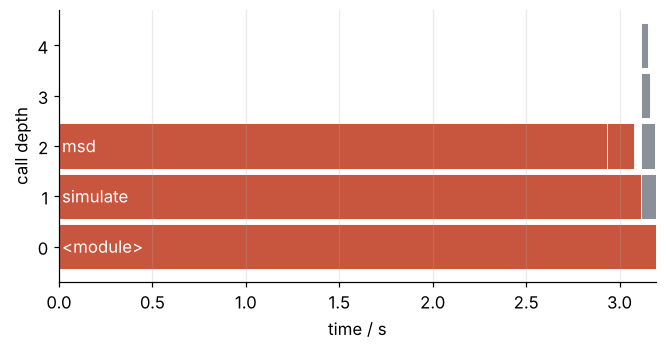
Flame graph of the slow run: time in s across, call depth up. Red bars are functions of walkers.py, gray bars Python itself. The msd bar covers nearly the whole run with nothing on top of it; the import of NumPy is a thin gray tower at the right.

The msd bar is nearly as wide as the run, and nothing sits on it: the bar is its own loop, the tottime of the table, plus callees under the cutoff. The gray tower at the right is NumPy's import, with the double counting squeezed out.

Step 5: Compare two runs on one time axis

Draw the run with the fix under the run without it, with sharex=True so both panels count the same seconds. The shared axis is the point: on its own axis each graph would fill its panel and look like a full run.

after = flame("after.prof")

fig, axes = plt.subplots(2, 1, sharex=True, figsize=(8, 4.4))
axes[0].set_xlim(0, 1.1 * before[0][2])        # room for the run time at the right
for ax, bars, name in zip(axes, [before, after], ["before", "after"]):
    draw(ax, bars)
    total = bars[0][2]
    ax.text(total, 0, f" {total:.2f} s", va="center", color=INK)
    ax.set_ylim(top=ax.get_ylim()[1] + 0.8)    # a free strip at the top for the name
    ax.text(0.99, 0.97, name, transform=ax.transAxes, ha="right", va="top", color=INK)
axes[1].set_xlabel("time / s")
plt.show()

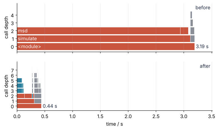
Flame graphs of the run before and after the fix, on one time axis in s. Red: functions of walkers.py; blue: NumPy; gray: Python itself. Before, the msd tower covers nearly the whole run of a few seconds; after, the whole run is a sliver of well under a second.

widest lists the chains with nothing on top, widest first, as shares of their run. A function with a slow loop of its own and one callee above the cutoff never appears on the list, since the callee sits on top; the uncovered part of its bar is its own time plus callees under the cutoff:

def widest(bars, n=5):
    """Print the n widest chains with nothing on top, as shares of the run."""
    chains = [c for c, _, _ in bars]
    tops = [(c, w) for c, _, w in bars if not any(d[:-1] == c for d in chains)]
    for chain, width in sorted(tops, key=lambda cw: -cw[1])[:n]:
        print(f"{100 * width / bars[0][2]:5.1f} %  " + " > ".join(label(f) for f in chain[1:]))

for name, bars in [("before", before), ("after", after)]:
    print(name)
    widest(bars)

before
 91.9 %  simulate > msd
  4.5 %  simulate > step
  1.1 %  _find_and_load > _find_and_load_unlocked > _load_unlocked > exec_module
after
 29.9 %  simulate > step
 19.4 %  simulate > msd_fast > sum > _wrapreduction > reduce
  4.9 %  _find_and_load > _find_and_load_unlocked > _load_unlocked > exec_module > _call_with_frames_removed > exec
  4.7 %  _find_and_load > _find_and_load_unlocked > _load_unlocked > exec_module > _call_with_frames_removed > __import__
  4.4 %  simulate > reflect

Before the fix, simulate > msd holds about nine tenths of the run. After it, step, which draws the random numbers, leads with about a third of the much shorter run, and NumPy's reduce inside msd_fast follows with about a fifth. Both already work on whole arrays, so by the stop rule of Profiling with cProfile and timeit there is little left to gain line by line; the fix itself is the subject of Vectorizing loops with NumPy. In the figure, the whole gray tower of the NumPy import, untouched by the fix, is now about a quarter of the run.

Pitfalls

A chain that never ran. In this short script prepare calls a helper run with load, and analyze calls it with smooth, the round-number case of Step 2:

%%writefile chains.py
def load(n):                     # stands in for reading data
    total = 0.0
    for i in range(n):
        total += 0.5 * i
    return total

def smooth(n):                   # stands in for filtering it, with the same amount of work
    total = 0.0
    for i in range(n):
        total -= 0.5 * i
    return total

def run(task, n):                # one helper, called from two places
    return task(n)

def prepare():
    return run(load, 5_000_000)

def analyze():
    return run(smooth, 5_000_000)

prepare()
analyze()

Writing chains.py

if not os.path.exists("chains.prof"):  # measures once for this page; drop this "if" in your copy
    subprocess.run([sys.executable, "-m", "cProfile", "-o", "chains.prof", "chains.py"], check=True)
widest(flame("chains.prof", script="chains.py"))

 27.0 %  analyze > run > smooth
 25.0 %  prepare > run > smooth
 25.0 %  analyze > run > load
 23.0 %  prepare > run > load

Two of these chains never happened, since analyze never ran load and prepare never ran smooth, and yet each gets about a quarter of the run. The split of Step 2 assumes that every call of a shared function did the same mix of work. Trust a chain only through functions with one caller, which the callers of Step 1 tell you. The viewers of a cProfile file have only the callers too. snakeviz gives each callee its whole edge under every chain and shrinks to fit, which for chains.py again draws the two chains that never ran, a quarter each; tuna stops at a function with several callers and draws its callees as one block of possible calls. When a shared helper matters, use a sampling profiler: it looks at the whole call stack many times a second and counts what it sees, so it never has to split.

Reading the x axis as a clock. You look for what ran first and find msd to the left of step, although every step of the simulation calls step first. Siblings are sorted by width, widest first, and the 2,000 calls of msd are merged into one bar, so left to right is not the order in time. Read the widths only. For the order of calls you need a tracer, a tool that logs every call and every return with its time stamp; a profile has thrown that away.

Profiling inside the notebook kernel. Profile code inside a Jupyter kernel and the table can hold rows that cannot be true. Profiling with cProfile and timeit found a function listed with less time than a function it calls, on Python 3.12 with ipykernel 7.4, and IPython's own functions can turn up among yours. A graph of such a profile should show a child wider than its parent. It does not: the shrink of Step 3 fits every child into its parent, so a wrong profile comes out as tidy as a sound one. The cause is the kernel's own background work, which cProfile records along with your code. Profile the script in its own process, as the setup does.

Variations

Icicle instead of flame. Call ax.invert_yaxis() after draw and the root moves to the top, the orientation snakeviz uses.
Color by change. Keep the before widths in a dict, {tuple(c): w for c, _, w in before}. Then color each bar of the after run by how much its chain grew or shrank, red for slower and blue for faster. This differential flame graph shows at once which chain a slowdown came from.
Explore it in the browser. snakeviz before.prof in a terminal opens the same file as an icicle or a sunburst in a local web page; tuna before.prof is a second viewer. Both start a web server, so neither runs on this page.
Whole stacks instead of callers. py-spy record -o profile.svg -- python walkers.py samples the run (Pitfall 1) and writes the flame graph as an SVG file, and pyinstrument walkers.py prints its samples as a call tree in the terminal.

Cheat sheet

# in a terminal: python -m cProfile -o before.prof walkers.py, then snakeviz before.prof
st = pstats.Stats("before.prof").stats           # (file, line, name) -> (cc, nc, tt, ct, callers)
callees = {}                                     # caller -> {callee: seconds on that edge}
for g, (cc, nc, tt, ct, callers) in st.items():  # callers: {f: (nc, cc, tt, ct)}, all calls first
    for f, edge in callers.items(): callees.setdefault(f, {})[g] = edge[3]
def walk(f, chain, left, width):                 # chain: the functions from the root to f
    ax.barh(len(chain) - 1, width, left=left)    # f's bar; ax.invert_yaxis() for an icicle
    share = width / st[f][3]                     # the part of f's time that came along this chain
    kids = {g: t * share for g, t in callees.get(f, {}).items() if g not in chain}  # the guard: no cycles
    fit = width / max(width, sum(kids.values()))  # the shrink; then walk each g at width kids[g] * fit