Zoom into a detail of a Matplotlib plot with an inset

The problem

You have a Matplotlib plot where a small feature sits next to a large one, and no single y range shows both. You want the whole plot plus an inset, a smaller Axes (one panel of a Matplotlib figure) magnifying the small feature, with a box and two lines that mark where it came from, legible in a paper. A log axis is no answer: it flattens the large peak and stretches the baseline noise until it rivals the small feature.

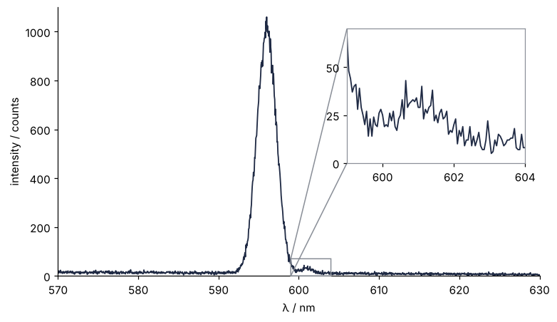
The example is an emission spectrum, a strong line of 1000 counts with a 20-count satellite 5 nm to its red side. A chromatogram or a fluorescence spectrum with a small peak on the tail of a large one is the same figure. Swap in your own data and zoom region.

The code

Copy

import numpy as np
import matplotlib.pyplot as plt

# ---- data: replace these lines with your own lam and counts
rng = np.random.default_rng(58)
lam = np.linspace(570, 630, 1201)                           # wavelength / nm, 0.05 nm steps

def line(lam, height, center, width):
    return height * np.exp(-0.5 * ((lam - center) / width) ** 2)

expected = 15 - 0.15 * (lam - 570) + line(lam, 1000, 596, 1.2) + line(lam, 20, 601, 0.7)
counts = rng.poisson(expected)                              # photon counting gives Poisson noise

# ---- zoom region and inset position
xlim, ylim = (570, 630), (0, 1100)                          # main axes, data units (nm, counts)
region = (599, 604, 0, 70)                                  # zoom region, data units: x0, x1, y0, y1
bounds = [0.60, 0.42, 0.37, 0.50]                           # inset: x0, y0, width, height in fractions of the main axes

# ---- main axes
INK, MUTED = "#1f2a44", "#8a8f98"
fig, ax = plt.subplots(figsize=(7, 4),                      # 7 in = 17.8 cm: printed 1:1, 10 pt stays 10 pt
                       dpi=110,                             # screen pixels per inch; the millimeters below do not depend on it
                       layout="constrained")                # shrink the axes until every label fits in the figure
ax.plot(lam, counts, color=INK, lw=1.2)
ax.set(xlim=xlim, ylim=ylim, xlabel="λ / nm", ylabel="intensity / counts")
ax.spines[["top", "right"]].set_visible(False)              # spines: the frame lines of an Axes

# ---- inset
inset = ax.inset_axes(bounds, xlim=region[:2], ylim=region[2:])
inset.plot(lam, counts, color=INK, lw=1.2)                  # a separate Axes: it shows only what is drawn into it
inset.locator_params(nbins=3)                               # fewer ticks, not smaller labels
inset.spines[:].set_color(MUTED)
# box and connecting lines, drawn from the inset's limits; the default alpha draws them half transparent
indicator = ax.indicate_inset_zoom(inset, edgecolor=MUTED, alpha=1)

# ---- report and plot
x0, y0, w, h = bounds
mag_x = w * (xlim[1] - xlim[0]) / (region[1] - region[0])
mag_y = h * (ylim[1] - ylim[0]) / (region[3] - region[2])
print(f"inset draws λ {mag_x:.1f}x and counts {mag_y:.1f}x as large as the main axes")

fx = (lam - xlim[0]) / (xlim[1] - xlim[0])                  # each point in fractions of the main axes (linear axes)
fy = (counts - ylim[0]) / (ylim[1] - ylim[0])
covered = (x0 < fx) & (fx < x0 + w) & (y0 < fy) & (fy < y0 + h)
print(f"data points under the inset: {covered.sum()}")

fig.canvas.draw()                                           # place the text, so its size is known
mm = 25.4 / fig.dpi                                         # pixels to millimeters
# Matplotlib also labels ticks just outside the view, so keep those inside;
# get_window_extent() is the box each label occupies
xlab = [t.get_window_extent() for v, t in zip(inset.get_xticks(), inset.get_xticklabels())
        if region[0] <= v <= region[1]]
ylab = [t.get_window_extent() for v, t in zip(inset.get_yticks(), inset.get_yticklabels())
        if region[2] <= v <= region[3]]
gap_x = min(b.x0 - a.x1 for a, b in zip(xlab, xlab[1:])) * mm   # side by side
gap_y = min(b.y0 - a.y1 for a, b in zip(ylab, ylab[1:])) * mm   # stacked
size = inset.get_xticklabels()[0].get_fontsize()
print(f"inset tick labels at {size:.0f} pt: {len(xlab)} on x, {gap_x:.0f} mm apart; "
      f"{len(ylab)} on y, {gap_y:.0f} mm apart")
plt.show()

inset draws λ 4.4x and counts 7.9x as large as the main axes
data points under the inset: 0
inset tick labels at 10 pt: 3 on x, 16 mm apart; 3 on y, 11 mm apart

The knobs

bounds places the inset: lower-left corner, width, and height in fractions of the main axes, so [0.60, 0.42, 0.37, 0.50] is the upper right; the first pitfall says where to put it. ax.inset_axes(bounds, transform=ax.transData) expects bounds in nm and counts instead (transData is Matplotlib's name for data units), and the first two printed lines, which assume fractions, go silently wrong. Keep fractions. region is the zoom in data units. The box follows the inset's limits, so it always outlines what the inset shows, in Matplotlib 3.11 even after they change. figsize is the printed size: 7 × 4 inches is 17.8 cm, about the two-column text width of Physical Review's REVTeX class (check your journal's guide). For one 8.6 cm column, set figsize=(3.4, 2.2): the constrained layout shrinks the axes and the inset with them, and the third printed line says whether the labels still fit. indicator.connectors holds the connecting lines to the inset's lower-left, upper-left, lower-right, and upper-right corners, and Matplotlib shows the first two. The lower one here cuts across a corner of the box, clear of the satellite, so I keep it; set_visible on an entry changes the pick. The inset is a full Axes, so a fit with its confidence band goes into it with the same calls.

The first printed line is the magnification on the page: the inset's share of the main axes times the ratio of the ranges, 0.37 × 60/5 = 4.4 in λ and 0.50 × 1100/70 = 7.9 in counts. In the inset the satellite's 20 counts look as tall as about 160 counts would in the main axes, so its height is read off the inset's tick labels, never off its look, and that is why the labels stay. The second line counts data points under the inset, and 0 is the number to keep when you move it. The third line measures the inset's tick labels on paper: three per axis at 10 pt, the size of the main ticks, 16 mm apart side by side on x and 11 mm stacked on y. About 2 mm, the width of one digit at 10 pt, keeps neighbors apart in either direction; at 0 they touch. The check holds only at the size the figure is built, which is the third pitfall's subject.

Pitfalls

An inset that covers data. Slide the inset left over the strong line and the line disappears behind it, with no warning. The inset is drawn at zorder 5, the drawing order in which higher draws on top, while the main axes' line sits at 2, and its face is opaque white. Put the inset in the corner where the data are lowest and check that the second printed line reads 0. If no corner is free, raise the upper limit in ylim until one is.

A box as tall as the plot. Give the inset only xlim, and the box on the main axes runs the full height of the plot while the satellite in the inset is a flat line near its floor. The inset autoscales y to all the data it holds, which is the whole spectrum up to the top of the strong line, not just the 5 nm it shows, and the box follows the inset's limits. Give both limits, as region does. The related slip is ax.set_xlim where inset.set_xlim was meant, which zooms the main axes instead.

Tick labels lost at print size. Delete the locator_params line and the third printed line shows the defaults: more tick labels, packed closer, in a panel a third as wide as the main axes. The usual remedy, tick_params(labelsize=6), makes them the smallest text on the figure, and a figure built at 7 inches and later shrunk into an 8.6 cm column prints at 0.48 of its size, so those labels end up at 2.9 pt. Ask for fewer ticks at full size with locator_params(nbins=3), build the figure at the width it will print, as the recipe's figsize does, and read the third printed line. Taking the labels off, as many examples do, is no fix, for the reason in the knobs. Line widths and fonts for the rest of a print figure are in the size step of the Matplotlib tutorial.