The L-shaped membrane with scipy.sparse: why the corner slows convergence

The problem

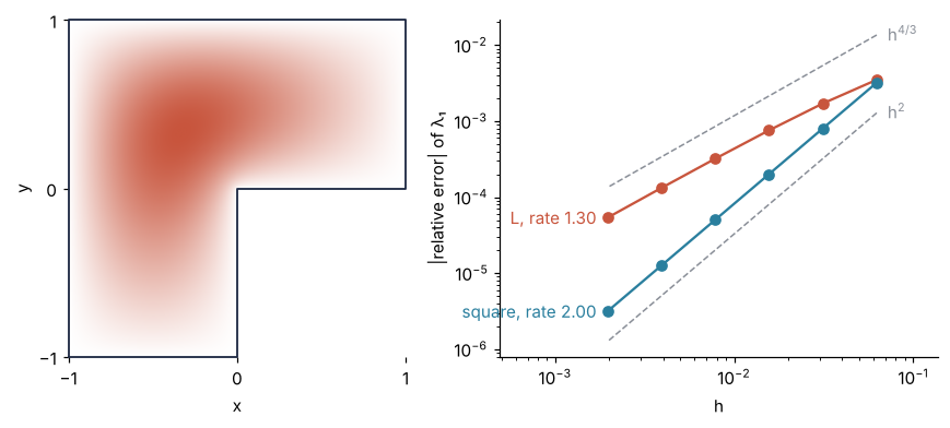
An L-shaped membrane, the square \([-1, 1]^2\) minus its lower right quadrant, clamped at the edge, has the lowest eigenvalue 9.6397238440219 of \(-\nabla^2\varphi = \lambda\varphi\) (Betcke and Trefethen, 2005). You want it from a grid with scipy.sparse and eigsh, as in Poisson's equation with scipy.sparse and Sparse eigenvalues with eigsh, and the rate \(p\) in error \(\propto h^p\): log2 of the error ratio per halving of the spacing \(h\). The unit square, rate 2, is the smooth control, and the L's third mode a check. The last column's rate, from differences of successive \(\lambda_1\), needs no reference.

Swap in your own grid-aligned shape: change the mask, the reference value, the grid's box, and the plotted outline.

The code

Copy

import numpy as np
import matplotlib.pyplot as plt
from matplotlib.colors import LinearSegmentedColormap
import scipy.sparse as sp
from scipy.sparse.linalg import eigsh

# ---- the five-point Laplacian and the lowest modes, as in the eigsh tutorial
def laplacian(n, h):
    D2, I = sp.diags_array([1.0, -2.0, 1.0], offsets=[-1, 0, 1], shape=(n, n)) / h**2, sp.eye_array(n)
    return (-(sp.kron(D2, I) + sp.kron(I, D2))).tocsr()

rng = np.random.default_rng(1967)
def lowest(A, k):
    return eigsh(A, k=k, sigma=0, v0=rng.standard_normal(A.shape[0]))

# ---- your shape: replace these two lines
def l_shape(X, Y): return ~((X >= 0) & (Y <= 0))    # nodes on the cut edges are clamped
LAM_L, LAM_SQ = 9.6397238440219, 2 * np.pi**2        # Betcke and Trefethen (2005) or np.nan; square

# ---- refine the grid: h = 1/m puts the corner and the cut edges on nodes
ms = [16, 32, 64, 128, 256, 512]
lam_L, lam_sq, n_L = [], [], []
for m in ms:
    h = 1 / m
    x = -1 + h * np.arange(1, 2 * m)                 # 2m - 1 interior points, x = 0 among them
    X, Y = np.meshgrid(x, x, indexing="ij")
    inside = l_shape(X, Y).ravel()
    A = laplacian(2 * m - 1, h)[inside][:, inside]
    lam, modes = lowest(A, 3)
    lam_L.append(lam[0]); n_L.append(A.shape[0])
    lam_sq.append(lowest(laplacian(m - 1, h), 1)[0][0])

# ---- rates: log2 of the error ratio per halving of h
err_L, err_sq = np.array(lam_L) / LAM_L - 1, np.array(lam_sq) / LAM_SQ - 1
rate_L, rate_sq = np.log2(err_L[:-1] / err_L[1:]), np.log2(err_sq[:-1] / err_sq[1:])
d = np.diff(lam_L)                                   # needs no reference value
rate_d = np.log2(d[:-1] / d[1:])

# ---- report and plot
print("   m  unknowns    λ₁ of L   rel. error  rate   square error  rate   rate from Δλ")
r = lambda a, j: f"{a[j]:5.2f}" if 0 <= j < len(a) else "     "   # blank where no rate exists yet
for i, m in enumerate(ms):
    print(f"{m:4d} {n_L[i]:9,d} {lam_L[i]:10.6f}  {err_L[i]:+9.1e}  {r(rate_L, i - 1)}"
          f"  {err_sq[i]:+11.1e}  {r(rate_sq, i - 1)}   {r(rate_d, i - 2)}")
print(f"λ₃ of L = {lam[2]:.6f} against 2π² = {LAM_SQ:.6f}, rel. error {lam[2] / LAM_SQ - 1:+.1e}")

INK, ACCENT, SECOND, MUTED = "#1f2a44", "#c8553d", "#2a7f9e", "#8a8f98"
mode = modes[:, 0] * np.sign(modes[:, 0].sum())      # the sign eigsh returns is arbitrary
image = np.full(inside.size, np.nan)
image[inside] = mode / mode.max()
fig, (ax0, ax1) = plt.subplots(1, 2, figsize=(8, 3.6), dpi=110, width_ratios=[1, 1.3])
ax0.imshow(image.reshape(2 * m - 1, -1).T, origin="lower", extent=[-1, 1, -1, 1],
           cmap=LinearSegmentedColormap.from_list("w", ["white", ACCENT]))
ax0.plot([-1, 0, 0, 1, 1, -1, -1], [-1, -1, 0, 0, 1, 1, -1], color=INK, lw=1.2, clip_on=False)
ax0.set(xlabel="x", ylabel="y", xticks=[-1, 0, 1], yticks=[-1, 0, 1])
hs = 1 / np.array(ms)
for err, rate, color, name in [(err_L, rate_L, ACCENT, "L"), (err_sq, rate_sq, SECOND, "square")]:
    ax1.loglog(hs, np.abs(err), "o-", color=color, ms=6)
    ax1.text(hs[-1] / 1.15, abs(err[-1]), f"{name}, rate {rate[-1]:.2f}", color=color, ha="right", va="center")
for p, k, err, label in [(4 / 3, 2.5, err_L, r"$\mathregular{h^{4/3}}$"), (2, 0.4, err_sq, r"$\mathregular{h^2}$")]:
    guide = k * abs(err[-1]) * (hs / hs[-1])**p      # 4/3 above the L, 2 below the square
    ax1.loglog(hs, guide, "--", color=MUTED, lw=1)
    ax1.text(hs[0] * 1.15, guide[0], label, color=MUTED, va="center")
ax1.set(xlabel="h", ylabel="|relative error| of λ₁", xlim=(hs[-1] / 4, hs[0] * 2.2))
ax0.spines[:].set_visible(False); ax1.spines[["top", "right"]].set_visible(False)   # the outline frames the L
fig.tight_layout()
plt.show()

   m  unknowns    λ₁ of L   rel. error  rate   square error  rate   rate from Δλ
  16       705   9.673506   +3.5e-03            -3.2e-03               
  32     2,945   9.656202   +1.7e-03   1.04     -8.0e-04   2.00        
  64    12,033   9.647023   +7.6e-04   1.17     -2.0e-04   2.00    0.91
 128    48,641   9.642810   +3.2e-04   1.24     -5.0e-05   2.00    1.12
 256   195,585   9.640996   +1.3e-04   1.28     -1.3e-05   2.00    1.22
 512   784,385   9.640240   +5.4e-05   1.30     -3.1e-06   2.00    1.26
λ₃ of L = 19.739147 against 2π² = 19.739209, rel. error -3.1e-06

The knobs

The spacing is \(h = 1/m\), so both cut edges and the re-entrant corner fall on nodes. It is the inner corner at the origin, where the membrane wraps 270° around the point. l_shape returns False on the clamped edge, hence the >= and <=, and the shape's edges must lie on grid lines: L, T, U, and cross shapes work, while a slanted edge becomes a staircase with rate 1, like the disk in the eigsh tutorial. sigma=0 finds the lowest modes because every eigenvalue of a clamped membrane is positive, and k=3 brings the next two tones along. The finest \(m\) sets the cost: each halving quadruples the unknowns, and the 784,385 at \(m\) = 512 take most of the cell's 40 s and 1.5 GB. For a shape with no published value, set LAM_L = np.nan, which blanks the error columns and the L's curve, and read the last column. If \(\lambda_h = \lambda + C h^p\), the differences \(\lambda_h - \lambda_{h/2}\) fall by the same \(2^p\) per halving. Their rate lags: 1.26 from the grids \(m\) = 128, 256, and 512, against 1.28 from the errors at \(m\) = 128 and 256, because a difference keeps 3/4 of the smooth \(h^2\) term but only 60 % of the corner's.

The square's error falls fourfold per halving, the \(h^2\) the stencil promises for a smooth mode. The L's falls about 2.5-fold, its rate climbing toward 4/3. Near a corner of opening angle \(\omega\), in polar coordinates \(r, \theta\) about it, a mode behaves like \(r^{\pi/\omega}\sin(\pi\theta/\omega)\). At 270° that is \(r^{2/3}\), whose slope is infinite at the corner, so the stencil's error bound, which assumes bounded derivatives, fails there. The eigenvalue error then falls like \(h^{2\pi/\omega}\), twice the corner exponent. Cleve Moler shows it at 270° for the five-point operator in his blog post MathWorks Logo, Part Two. Finite Differences. A grid-aligned shape without slits can have only 270° re-entrant corners. Expect 4/3 if your shape has one and 2 if it has none. The L comes out high and the square low. The corner's term pushes \(\lambda\) up, the smooth \(h^2\) part pulls it down and fades faster, so the rate approaches 4/3 from below. None of this is eigsh: the matrix eigenvalue is exact to rounding, and the error is the grid's.

Pitfalls

A corner or an edge between the nodes. The error halves with every halving of \(h\), and \(\lambda_1\) comes out low. The clamped boundary sits half a spacing to a full spacing outside the true edge, which makes the membrane larger. It happens with np.linspace(-1, 1, n) and an even n, which misses \(x = 0\), or with a strict mask that keeps the nodes on the cut edges as unknowns:

for m in [64, 128]:
    h = 1 / m
    x = -1 + h * np.arange(1, 2 * m)
    X, Y = np.meshgrid(x, x, indexing="ij")
    for name, keep in [("strict", ~((X > 0) & (Y < 0))), ("l_shape", l_shape(X, Y))]:
        keep = keep.ravel()
        lam = lowest(laplacian(2 * m - 1, h)[keep][:, keep], 1)[0][0]
        print(f"m = {m:3d}  {name:7s}  λ₁ − λ = {lam - LAM_L:+.4f}  ({lam / LAM_L - 1:+.2%})")

m =  64  strict   λ₁ − λ = -0.2534  (-2.63%)
m =  64  l_shape  λ₁ − λ = +0.0073  (+0.08%)
m = 128  strict   λ₁ − λ = -0.1289  (-1.34%)
m = 128  l_shape  λ₁ − λ = +0.0031  (+0.03%)

The strict mask is low by 0.25 at \(m\) = 64 and by 0.13 at \(m\) = 128, halving, while l_shape is high by 0.0073 and 0.0031. Pick a spacing that divides every edge length and clamp the edge nodes with >= and <=.

A rate from two coarse grids. The first halving gives 1.04, which reads as first order and a bug. The rate settles only on the finer grids, at 1.28 and 1.30, because on coarse grids the smooth \(h^2\) part of the error is still comparable with the corner's. Print the rate of every halving and quote the last ones once they stop moving.

Testing on a smooth mode. The third eigenvalue of the L is exactly \(2\pi^2\), the mode \(\sin\pi x \sin\pi y\), which vanishes along the cut lines and is a sine mode on each of the three squares. It never sees the corner and converges like the square: its relative error at \(m\) = 512 is −3.1e-6, the square's own. A check against \(\lambda_3\) passes and hides the corner. Check the convergence of the mode you need, here \(\lambda_1\), because the modes that feel the corner are the ones that are not smooth there.