Sparse eigenvalues with scipy.sparse.linalg.eigsh: the tones of a drum
Afterwards you can build a sparse matrix from a stencil, get its lowest eigenvalues and eigenvectors with eigsh and shift-invert, and check them on exact cases.
- Field
- Engineering, Mathematics, Physics
- Libraries
matplotlib 3.11.2numpy 2.5.3scipy 1.18.1
py-scipy-sparse-eigsh.ipynb, executed with the versions above. The download needs a free account
Run it yourself. In a terminal, this installs exactly the versions above:
pip install numpy==2.5.3 scipy==1.18.1 matplotlib==3.11.2 jupyterlabThe problem: why a drum does not sound like a note
Pluck a string and its overtones come at 2, 3, and 4 times the lowest frequency, which is what makes a note. Strike a circular drum and they come at 1.593, 2.136, and 2.295 times the lowest, ratios of zeros of Bessel functions with no whole numbers hiding in them. The drum is not out of tune. It has no tune to be in.
A drumhead clamped at its rim obeys the wave equation \(\partial_t^2 u = c^2\nabla^2 u\), and a standing wave \(u = \varphi(x, y)\cos\omega t\) turns it into an eigenvalue problem,
with \(\varphi = 0\) on the rim. The ratio of two frequencies is the square root of the ratio of their eigenvalues, and the wave speed \(c\) drops out.
On a grid of 200 by 200 points, \(-\nabla^2\) becomes a matrix with 40,000 rows. Stored dense it takes 12.8 GB, stored sparse 2.6 MB. In Eigenvalues with numpy.linalg you found the modes of three masses with a dense solver. From three masses to forty thousand you need scipy.sparse.linalg.eigsh, which finds a few eigenvalues of a large sparse symmetric matrix, here the six lowest, without ever forming the dense one.
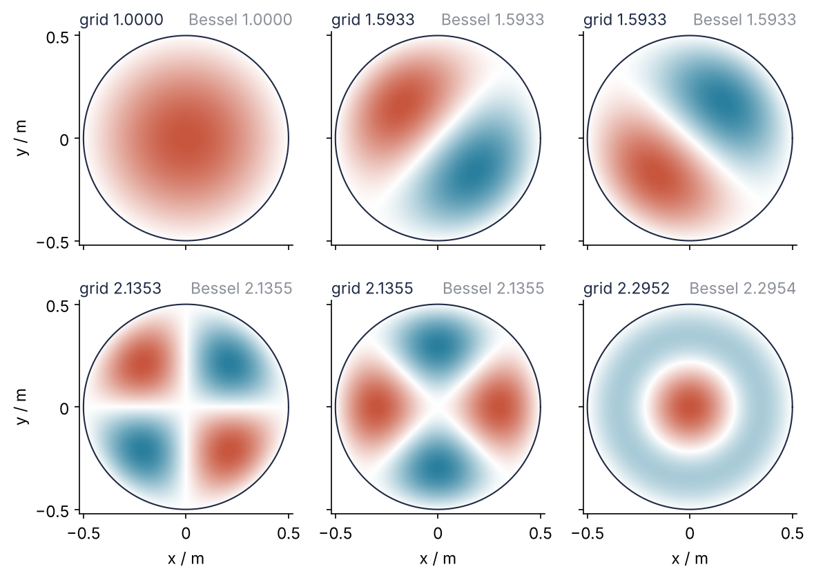
These are the first six modes of a circular drum, each panel one eigenvector from eigsh, labeled with its frequency ratio from the grid and the exact value from Bessel zeros. Six steps lead there, by way of a square drum whose tones are known exactly.
Setup
One grid serves both drums: a square of side \(L\) = 1 m with \(N\) = 200 interior points per side, and later the circle inscribed in it. The random generator seeds the start vectors of eigsh, so a rerun on your machine repeats every result below.
import numpy as np
import matplotlib.pyplot as plt
from matplotlib.colors import LinearSegmentedColormap
import scipy.sparse as sp
from scipy.sparse.linalg import eigsh, splu, LinearOperator
from scipy.special import jn_zeros, jv

L = 1.0              # m, side of the square
N = 200              # interior grid points per side
h = L / (N + 1)      # m, grid spacing
R = L / 2            # m, radius of the circular drum
rng = np.random.default_rng(2026)

plt.rcParams.update({                      # the look of every figure below
    "figure.figsize": (7, 3.6), "figure.dpi": 110,
    "axes.spines.top": False, "axes.spines.right": False,
    "axes.grid": True, "grid.alpha": 0.25,
    "font.size": 11, "lines.linewidth": 1.8,
})
INK, ACCENT, SECOND, MUTED = "#1f2a44", "#c8553d", "#2a7f9e", "#8a8f98"
DRUM = LinearSegmentedColormap.from_list("drum", [SECOND, "white", ACCENT])

print(f"h = {1e3 * h:.3f} mm, {N * N:,} unknowns")
h = 4.975 mm, 40,000 unknowns
Step 1: Build the second difference with diags_array
The second derivative of a function sampled at spacing \(h\) is approximately \((u_{i-1} - 2u_i + u_{i+1})/h^2\), with an error that shrinks as \(h^2\). Applied to every point of a string at once, this is a matrix with \(-2\) on the diagonal and 1 on its two neighbors, divided by \(h^2\). diags_array builds it from the three diagonals:
def second_difference(n, h):
    return sp.diags_array([1.0, -2.0, 1.0], offsets=[-1, 0, 1], shape=(n, n)) / h**2

print(second_difference(5, 1.0).toarray())
[[-2.  1.  0.  0.  0.]
 [ 1. -2.  1.  0.  0.]
 [ 0.  1. -2.  1.  0.]
 [ 0.  0.  1. -2.  1.]
 [ 0.  0.  0.  1. -2.]]
The first and last rows have only two entries. The missing third would multiply a point beyond the end, which is held at zero: the clamped ends are in the matrix although no line of code mentions them. At 200 unknowns the dense eigh you know still works, or eigvalsh, which skips the eigenvectors. Check the claim about strings:
lam_string = np.linalg.eigvalsh((-second_difference(N, h)).toarray())
print("frequency ratios:", np.round(np.sqrt(lam_string[:4] / lam_string[0]), 4))
frequency ratios: [1. 1.9999 2.9998 3.9994]
The harmonics 1, 2, 3, 4, to three or four digits.
Step 2: Assemble the drum's Laplacian with kron and store it as CSR
On an \(n \times n\) grid, number the points so that point \((i, j)\) is entry \(k = i\,n + j\) of the vector: the \(n\) points that share an \(i\) sit next to each other. The Kronecker product replaces each entry of one matrix by that entry times the whole of another,
In kron(\(D_2\), \(I\)) every entry of \(D_2\) becomes a multiple of the identity, which couples point \((i, j)\) to \((i \pm 1, j)\): the second difference in \(i\). In kron(\(I\), \(D_2\)) copies of \(D_2\) sit in the diagonal blocks and couple \((i, j \pm 1)\), the second difference in \(j\). Their sum is the five-point Laplacian, and the minus sign makes the eigenvalues positive, \(\lambda = (\omega/c)^2\). On a 3 × 3 grid, times \(h^2\):
def laplacian(n, L):
    h = L / (n + 1)
    D2, I = second_difference(n, h), sp.eye_array(n)
    return (-(sp.kron(D2, I) + sp.kron(I, D2))).tocsr()

print((laplacian(3, L) * (L / 4)**2).toarray().astype(int))
[[ 4 -1  0 -1  0  0  0  0  0]
 [-1  4 -1  0 -1  0  0  0  0]
 [ 0 -1  4  0  0 -1  0  0  0]
 [-1  0  0  4 -1  0 -1  0  0]
 [ 0 -1  0 -1  4 -1  0 -1  0]
 [ 0  0 -1  0 -1  4  0  0 -1]
 [ 0  0  0 -1  0  0  4 -1  0]
 [ 0  0  0  0 -1  0 -1  4 -1]
 [ 0  0  0  0  0 -1  0 -1  4]]
Each row has 4 on the diagonal and \(-1\) for every neighbor. Row 2, the point (0, 2), has no \(-1\) in column 3, the point (1, 0): they are adjacent in the numbering but not on the grid, and the Kronecker structure puts that zero in for free.
sp.kron returns COO, a list of (row, column, value) triples, quick to build and slow to compute with. The sum of two such terms comes back as CSR; a single one stays COO. .tocsr() costs nothing on CSR and keeps the matrix CSR if you change the sum. CSR keeps three arrays: data holds the nonzero values row by row, indices the column of each, and indptr, one entry longer than there are rows, where each row starts in the other two.
A = laplacian(N, L)
D2, I = second_difference(N, h), sp.eye_array(N)
print("format of one kron:", sp.kron(D2, I).format, "  of the sum:", (sp.kron(D2, I) + sp.kron(I, D2)).format)

sparse_bytes = A.data.nbytes + A.indices.nbytes + A.indptr.nbytes
print(f"A: {A.format}, {A.shape[0]:,} × {A.shape[1]:,}, {A.nnz:,} nonzeros")
print(f"data {A.data.nbytes:,} + indices {A.indices.nbytes:,} + indptr {A.indptr.nbytes:,} = {sparse_bytes:,} bytes")
print(f"dense: {A.shape[0]**2 * 8:,} bytes")
format of one kron: coo   of the sum: csr
A: csr, 40,000 × 40,000, 199,200 nonzeros
data 1,593,600 + indices 796,800 + indptr 160,004 = 2,550,404 bytes
dense: 12,800,000,000 bytes
Five nonzeros per row, less the 800 neighbors missing at the edges: 2.6 MB against 12.8 GB, 5,000 times less.
Step 3: Ask eigsh for the lowest tones
eigsh runs ARPACK's Lanczos method, which touches the matrix only through products \(A\mathbf x\). Write \(\mathbf x\) in eigenvectors and each product multiplies the component along \(\mathbf v_k\) by \(\lambda_k\), so repeated products grow the components with the largest \(|\lambda|\) fastest. Lanczos makes the best use of every vector it has produced, but the bias stays. Asking for the smallest with which="SM" works, and it is slow. To see how slow, hand eigsh a LinearOperator, which it accepts in place of a matrix and which is defined only by what it does to a vector. The short form is LinearOperator(A.shape, matvec=f), with f(x) returning the product. A subclass that overrides _matvec, the method behind every product, can count its calls as well.
class Counted(LinearOperator):
    """Apply a function to a vector and count how often that happens."""
    def __init__(self, apply, shape):
        super().__init__(dtype=float, shape=shape)
        self.apply, self.calls = apply, 0

    def _matvec(self, x):
        self.calls += 1
        return self.apply(x)

v0 = rng.standard_normal(A.shape[0])
products = Counted(lambda x: A @ x, A.shape)
vals, vecs = eigsh(products, k=6, which="SM", v0=v0)
print(f"{products.calls:,} products")
print("λ / m⁻²:", np.round(vals, 4))
6,162 products
λ / m⁻²: [19.7388 49.3446 49.3446 78.9504 98.6796 98.6796]
Several thousand products for six numbers. The wanted eigenvalues, 20 to 100 m⁻², sit close together at the bottom of a spectrum that reaches nearly \(8/h^2 \approx 3.2 \times 10^5\) m⁻². The count will not be the same on your machine. It depends on rounding in the BLAS library underneath SciPy, which changes with the number of threads and with the BLAS kernel chosen for the CPU: here between 6,162 and 8,177 over one to four threads and four kernels, with the same six eigenvalues every time. The same rounding moved Step 4's 54 solves to 55 with one kernel, and it decides which rotated copy of a degenerate pair of modes comes back, as Pitfall 3 shows. Put %time in front of the call to see what the products cost on yours.
Step 4: Shift-invert: factor once, solve fifty times
Turn the spectrum around. If \(A\mathbf v = \lambda\mathbf v\), then \((A - \sigma I)\mathbf v = (\lambda - \sigma)\mathbf v\), so
the same eigenvectors, with eigenvalues \(1/(\lambda - \sigma)\). The \(\lambda\) nearest \(\sigma\) become the largest in magnitude and the best separated, which is what Step 3's products find fast. With \(\sigma = 0\) that is \(A^{-1}\), and nearest zero means lowest only because every eigenvalue of the clamped drum is positive.
The inverse is never formed. It has no zero entries, since every point of a clamped drum responds to a push at any other point, so it would take 12.8 GB again. Instead splu factors \(A - \sigma I\), here \(A\), once into a lower and an upper triangle, the bookkeeping of Gaussian elimination kept for reuse. Elimination fills in some of the zeros of \(A\), but the triangles stay sparse. Applying the inverse to a vector is then one lu.solve, a forward and a back substitution. splu wants CSC, the same three arrays stored column by column; given CSR it converts and warns. With OPinv set, eigsh never multiplies by \(A\), and a second counter on \(A\) shows it.
lu = splu(A.tocsc())
solves = Counted(lu.solve, A.shape)
products = Counted(lambda x: A @ x, A.shape)
vals, vecs = eigsh(products, k=6, sigma=0, OPinv=solves, v0=v0)
print(f"{solves.calls} solves, {products.calls} products")
print("λ / m⁻²:", np.round(vals, 4))

factor_nnz = lu.L.nnz + lu.U.nnz
print(f"nonzeros in L and U: {factor_nnz:,} = {factor_nnz / A.nnz:.1f} × A.nnz")
print(f"{solves.calls} solves touch as many numbers as {solves.calls * factor_nnz / A.nnz:.0f} products")
54 solves, 0 products
λ / m⁻²: [19.7388 49.3446 49.3446 78.9504 98.6796 98.6796]
nonzeros in L and U: 3,472,176 = 17.4 × A.nnz
54 solves touch as many numbers as 941 products
Fifty-four solves, the same six eigenvalues, and not one product. Do not read several thousand products against 54 solves as a hundredfold gain. A solve touches 17 times as many stored numbers as a product, so the solves are worth about 940 products, and the factorization comes on top, paid once.
eigsh(A, k=6, sigma=0) builds the same factorization itself:
vals_auto, vecs_auto = eigsh(A, k=6, sigma=0, v0=v0)
print("largest difference to the hand-built version:", np.abs(vals_auto - vals).max())
largest difference to the hand-built version: 0.0
With sigma set, which keeps its default "LM" but applies to \(1/(\lambda - \sigma)\), and eigsh hands back \(\lambda\) itself, sorted from lowest to highest.
Step 5: Check the square drum against its exact tones
The square has an exact answer: modes \(\sin(m\pi x/L)\sin(n\pi y/L)\) with \(\lambda = \pi^2(m^2 + n^2)/L^2\) for \(m, n \ge 1\). The six lowest are (1,1), (1,2), (2,1), (2,2), (1,3), and (3,1).
lam = vals_auto
mn = np.array([(1, 1), (1, 2), (2, 1), (2, 2), (1, 3), (3, 1)])
lam_exact = np.pi**2 * (mn**2).sum(axis=1) / L**2

print("m,n   λ grid    λ exact   rel. error   ratio grid  exact")
for (m, n), lg, le in zip(mn, lam, lam_exact):
    print(f"{m},{n}  {lg:9.4f}  {le:9.4f}   {lg / le - 1:+.1e}      "
          f"{np.sqrt(lg / lam[0]):.4f}   {np.sqrt(le / lam_exact[0]):.4f}")
m,n   λ grid    λ exact   rel. error   ratio grid  exact
1,1    19.7388    19.7392   -2.0e-05      1.0000   1.0000
1,2    49.3446    49.3480   -6.9e-05      1.5811   1.5811
2,1    49.3446    49.3480   -6.9e-05      1.5811   1.5811
2,2    78.9504    78.9568   -8.1e-05      1.9999   2.0000
1,3    98.6796    98.6960   -1.7e-04      2.2359   2.2361
3,1    98.6796    98.6960   -1.7e-04      2.2359   2.2361
Every eigenvalue comes out a little low, the fundamental by 2.0e-5 and the (1,3) mode by 1.7e-4, and the ratios agree to three or four digits. The pairs (1,2) and (2,1) are equal to every printed digit, as the symmetry demands. The eigenvalues are in m⁻² because the matrix carries the \(1/h^2\) of Step 1; without it they would be 40,401 times smaller and comparable with nothing.
Step 6: Cut out a circular drum and look at its modes
Give every grid point its coordinates, centered on the square, in Step 2's order, and keep the points inside the circle of radius \(R\). Deleting the rows and columns of the rest clamps the drum at the staircase of grid points along the circle, as you clamped a fixed atom in the prerequisite.
The exact modes of the disk are \(J_m(j_{mk}r/R)\) times \(\cos m\theta\) or \(\sin m\theta\), with \(m\) nodal diameters and \(j_{mk}\) the \(k\)-th zero of the Bessel function \(J_m\), so that the rim is a node, and \(\lambda = (j_{mk}/R)^2\). jn_zeros(m, k) returns the first \(k\) positive zeros of \(J_m\). The six lowest are \(j_{01}\), then \(j_{11}\) and \(j_{21}\) twice each, once with the cosine and once with the sine, then the ring, \(j_{02}\) = 5.520, below \(j_{31}\) = 6.380.
def coordinates(n):
    x = -L / 2 + L / (n + 1) * np.arange(1, n + 1)
    X, Y = np.meshgrid(x, x, indexing="ij")     # i runs along x, as in Step 2's numbering
    return X.ravel(), Y.ravel()

def lowest(M, k):
    return eigsh(M, k=k, sigma=0, v0=rng.standard_normal(M.shape[0]))

X, Y = coordinates(N)
inside = X**2 + Y**2 < R**2
A_disk = A[inside][:, inside]
lam_disk, modes = lowest(A_disk, 6)

j = np.array([jn_zeros(0, 1)[0], *jn_zeros(1, 1), *jn_zeros(1, 1),
              *jn_zeros(2, 1), *jn_zeros(2, 1), jn_zeros(0, 2)[1]])
ratio_grid, ratio_bessel = np.sqrt(lam_disk / lam_disk[0]), j / j[0]
print(f"{A_disk.shape[0]:,} unknowns")
print("grid:  ", np.round(ratio_grid, 4))
print("Bessel:", np.round(ratio_bessel, 4))
31,700 unknowns
grid:   [1.     1.5933 1.5933 2.1353 2.1355 2.2952]
Bessel: [1.     1.5933 1.5933 2.1355 2.1355 2.2954]
There is the drum from the opening, 1.5933, 2.1353, 2.2952 against 1.5933, 2.1355, 2.2954. The grid splits the 2.136 pair into 2.1353 and 2.1355, as Pitfall 3 explains. Now both shapes at three resolutions:
print("   N   square λ₁ error   disk λ₁ error   disk ratio error")
for n in [50, 100, 200]:
    An = laplacian(n, L)
    err_square = lowest(An, 1)[0][0] / (2 * np.pi**2 / L**2) - 1
    Xn, Yn = coordinates(n)
    keep = Xn**2 + Yn**2 < R**2
    lam_n, _ = lowest(An[keep][:, keep], 6)
    err_disk = lam_n[0] / (j[0] / R)**2 - 1
    err_ratio = np.abs(np.sqrt(lam_n / lam_n[0]) - ratio_bessel).max()
    print(f"{n:4d}   {err_square:+15.1e}   {err_disk:+13.1e}   {err_ratio:16.1e}")
   N   square λ₁ error   disk λ₁ error   disk ratio error
  50          -3.2e-04        -2.4e-02            4.4e-03
 100          -8.1e-05        -1.3e-02            1.6e-03
 200          -2.0e-05        -6.4e-03            2.5e-04
The \(\lambda_1\) errors are relative and signed, the last column the worst ratio. The square's error falls fourfold per halving of \(h\), the \(h^2\) of Step 1; the disk's only twofold, because the staircase costs one order. The staircase lowers all tones together, as if the drum were a third of a grid spacing larger, and the shift cancels in the ratios: at \(N\) = 200 the fundamental is 0.64 % low, while no ratio is off by more than 2.5e-4.
fig, axes = plt.subplots(2, 3, figsize=(8, 5.8), sharex=True, sharey=True)
edge = L / 2 - h / 2
circle = np.linspace(0, 2 * np.pi, 400)
for k, ax in enumerate(axes.flat):
    mode = modes[:, k] * np.sign(modes[np.abs(modes[:, k]).argmax(), k])   # largest value positive
    image = np.full(N * N, np.nan)
    image[inside] = mode
    vmax = np.abs(mode).max()
    ax.imshow(image.reshape(N, N).T, origin="lower", extent=[-edge, edge, -edge, edge],
              cmap=DRUM, vmin=-vmax, vmax=vmax)
    ax.plot(R * np.cos(circle), R * np.sin(circle), color=INK, lw=1)
    ax.text(0, 1.03, f"grid {ratio_grid[k]:.4f}", color=INK, transform=ax.transAxes)
    ax.text(1, 1.03, f"Bessel {ratio_bessel[k]:.4f}", color=MUTED, ha="right", transform=ax.transAxes)
    ax.set(xlim=(-0.52, 0.52), ylim=(-0.52, 0.52), xticks=[-0.5, 0, 0.5], yticks=[-0.5, 0, 0.5],
           xticklabels=["−0.5", "0", "0.5"], yticklabels=["−0.5", "0", "0.5"])
    ax.grid(False)
for ax in axes[1]:
    ax.set_xlabel("x / m")
for ax in axes[:, 0]:
    ax.set_ylabel("y / m")
fig.tight_layout()
plt.show()
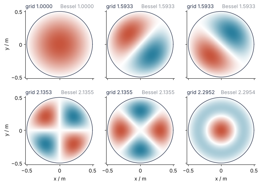
The colormap DRUM is white at zero, so the white diameters in a panel count its \(m\).
Pitfalls
A COO matrix where CSR belongs. The slicing A[inside][:, inside] of Step 6 takes milliseconds on CSR. On the COO array of a single kron it took about a minute here, because COO must search its triples for every row you ask for. A single kron, scaled or not, stays COO, which is why Step 2 calls .tocsr() even on the sum. Convert once after assembly, or ask for sp.kron(B, C, format="csr").
sigma=0 on a spectrum that is not all positive. Add a potential well, \(-\nabla^2 + V\) with \(V < 0\) in a small region, and eigsh(..., sigma=0) returns six eigenvalues near zero without complaint, while the deepest states, the ones you wanted, are missing. Nearest zero is lowest only for an all-positive spectrum, as Step 4 showed. A free edge fails for the same reason: its constant mode has \(\lambda = 0\), like the free molecule of the prerequisite, so \(A - \sigma I\) is singular. splu then raises "Factor is exactly singular" or, when rounding leaves a tiny pivot, carries on by luck. Put sigma a little below the lowest eigenvalue you want: below V.min() for a well, since \(-\nabla^2\) alone has only positive eigenvalues, and a small negative number such as \(-1\) for a free edge.
Degenerate pairs come back rotated. The two modes at 1.593 do not look like the textbook patterns \(J_1(j_{11}r/R)\cos\theta\) and \(\sin\theta\), and another seed or another machine turns them by another angle. Any two orthonormal combinations of a degenerate pair are eigenvectors, and eigsh returns whichever its start vector and the rounding led to. Compare the pair's span, not single vectors, with the projections \(c = V^\mathsf{T}\mathbf x\) of the prerequisite:
r, theta = np.hypot(X, Y)[inside], np.arctan2(Y, X)[inside]
textbook = jv(1, j[1] * r / R) * np.cos(theta)
textbook /= np.linalg.norm(textbook)
c = modes[:, 1:3].T @ textbook
print("projections on the two modes:", np.round(c, 3), f"  norm in their span: {np.linalg.norm(c):.4f}")
split = (lam_disk[[2, 4]] - lam_disk[[1, 3]]) / lam_disk[[1, 3]]
print(f"relative split of the pairs: 1.593 {split[0]:.0e}, 2.136 {split[1]:.1e}")
projections on the two modes: [0.735 0.678]   norm in their span: 1.0000
relative split of the pairs: 1.593 9e-15, 2.136 2.1e-04
Neither projection is near 1, and both change with the machine: over the runs of Step 3 they ranged from 0.685 and 0.729 to 0.785 and 0.619. Their norm was 1.0000 in every run. Neither mode is the pattern, yet their span holds all of it. The 1.593 pair is degenerate to a relative split of about 1e-14, so rounding alone picks its angle, but the grid splits the 2.136 pair by 2.1e-4 and so fixes its orientation: nodal lines along the grid lines in one mode, along the diagonals in the other.
Variations
- Another drum shape. The one change is
inside: an L-shaped mask, or the two drums of Gordon, Webb, and Wolpert, different shapes with the same eigenvalues (on a grid only nearly the same), which answer Kac's question "Can one hear the shape of a drum?" with no. - A quantum particle in a 2D box. \(\hbar^2/2m\) times
Aplussp.diags_array(V.ravel()), andsigmabelowV.min()as in Pitfall 2; the call is otherwise the same. - lobpcg with a preconditioner. For matrices too large to factor,
scipy.sparse.linalg.lobpcg(A, X, M=..., largest=False)with a blockXof six seeded random vectors finds the lowest modes withoutsplu. - A vibrating plate.
A @ Aon the square with simply supported edges has the eigenvalues \(\lambda^2\), so its frequency ratios are \((m^2 + n^2)/2\): 1, 2.5, 2.5, 4.
Cheat sheet
D2 = sp.diags_array([1.0, -2.0, 1.0], offsets=[-1, 0, 1], shape=(n, n)) / h**2   # clamped ends
A = (-(sp.kron(D2, I) + sp.kron(I, D2))).tocsr()      # five-point -∇², always CSR
vals, vecs = eigsh(A, k=6, sigma=0, v0=v0)           # sigma below the lowest you want; vals ascending
vals, vecs = eigsh(A, k=6, which="SM", v0=v0)        # same answer, thousands of products: slow
lu = splu(A.tocsc())                                 # factor once ...
OPinv = LinearOperator(A.shape, matvec=lu.solve)     # ... and hand eigsh the solves
A_mask = A[mask][:, mask]                            # clamp at the edge of any shape
ratios = np.sqrt(vals / vals[0])                     # frequency ratios
image = np.full(n * n, np.nan); image[mask] = vecs[:, k]   # a mode, ready for imshow
Further reading
scipy.sparse.linalg.eigshreference, in particular the notes onsigmaandwhich, and the SciPy guide to sparse arrays.- Lehoucq, Sorensen, Yang, ARPACK Users' Guide (SIAM, 1998), for implicitly restarted Lanczos and shift-invert.
- M. Kac, "Can one hear the shape of a drum?", American Mathematical Monthly 73 (1966), and Morse and Ingard, Theoretical Acoustics, for the vibrating membrane and its Bessel modes.
- Related tutorials on this site: Eigenvalues with numpy.linalg: normal modes of coupled oscillators; Solve a linear system with NumPy: the currents in a resistor network; The wave equation with leapfrog finite differences: a pulse on a string, the same second difference in time; findiff.PDE with mixed boundary conditions: seepage under a dam, another sparse matrix from a stencil.
- Download the notebook. It was executed with the library versions in the header.