Poisson's equation with scipy.sparse: two plates in a grounded box

The problem: the potential between two plates in a grounded box

A square box 10 cm on a side has grounded metal walls. Inside it stand two parallel plates, each 4 cm long and 30.7 mm apart, one held at +1 V and the other at −1 V. Between infinite plates the field would be ΔV/d, 65.2 V/m for this gap. These plates are short and the walls are close, so how much of that is left at the center? There is no charge in the box, so the potential φ obeys Laplace's equation, which is Poisson's equation \(\nabla^2\varphi = -\rho/\varepsilon_0\) with ρ = 0. On a grid of 100 × 100 nodes it becomes 10,000 linear equations, each tying a node to its four neighbors. The matrix of that system is almost all zeros, a sparse matrix, and scipy.sparse stores only the rest.

The same equation, with other names on the variables, gives steady heat flow in a plate and the groundwater head under a dam; findiff.PDE with mixed boundary conditions: seepage under a dam solves the second with a library that builds the matrix for you. Here you build it yourself. Solve a linear system with NumPy: the currents in a resistor network solved a handful of nodes with a dense matrix, and that does not scale to a grid this fine. Step 2 puts numbers on why.

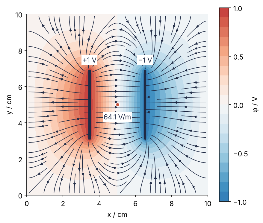
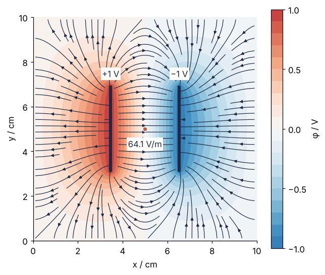
The finished result: the potential in the RdBu_r colormap, red positive and blue negative, and the field lines on top of it. At the center the field is 64.1 V/m, 1.6 % below the ideal value. One call to spsolve gives the potential, and np.gradient and streamplot the rest.

Setup

Lengths are in meters and potentials in volts. The walls sit one spacing outside the outermost nodes, so h = L/(N + 1).

import numpy as np
import scipy.sparse as sp
from scipy.sparse.linalg import spsolve, splu
import matplotlib.pyplot as plt

L = 0.10          # side of the box, m
N = 100           # nodes along each side
h = L / (N + 1)   # spacing; the walls are one spacing outside the outermost nodes

plt.rcParams.update({
    "figure.figsize": (6.5, 5.6), "figure.dpi": 110,
    "axes.spines.top": False, "axes.spines.right": False,
    "axes.grid": True, "grid.alpha": 0.25,
    "font.size": 11, "lines.linewidth": 1.8,
})
INK, ACCENT, SECOND, MUTED = "#1f2a44", "#c8553d", "#2a7f9e", "#8a8f98"

print(f"N x N = {N * N:,} nodes, h = {h * 1e3:.3f} mm")

N x N = 10,000 nodes, h = 0.990 mm

Step 1: Number the grid nodes into one vector

A linear system wants one vector of unknowns, and the potential lives on a 2D grid. NumPy flattens an array row by row, in C order: ravel turns the grid into a vector and reshape folds it back. On a small array whose entries are their own position in the vector:

labels = np.arange(12).reshape(3, 4)
print(labels)
print("node (1, 2) is entry", labels.ravel()[1 * 4 + 2])

[[ 0  1  2  3]
 [ 4  5  6  7]
 [ 8  9 10 11]]
node (1, 2) is entry 6

Node (i, j) of a grid with N columns is entry k = iN + j. Neighbors in j sit next to each other in the vector, and neighbors in i sit N entries apart, four in this example. Build the grid with indexing="ij", so that axis 0 is x and axis 1 is y:

x = h * np.arange(1, N + 1)
X, Y = np.meshgrid(x, x, indexing="ij")
print(f"node (1, 0) sits at x = {X[1, 0] * 1e3:.2f} mm, y = {Y[1, 0] * 1e3:.2f} mm")

node (1, 0) sits at x = 1.98 mm, y = 0.99 mm

Moving one step along axis 0 moves you along x. Neighbors along y are therefore adjacent in the vector, neighbors along x are N entries apart, and the matrix will have bands at offsets ±1 and ±N. The seepage tutorial numbered its nodes the same way.

Step 2: Build the five-point Laplacian with diags_array and kron

The wave equation with leapfrog finite differences: a pulse on a string used the second difference \((u_{j-1} - 2u_j + u_{j+1})/h^2\). For all N nodes on a line it is one tridiagonal matrix D, with 1, −2, 1 on its three central diagonals, divided by h². The first row has no \(u_{j-1}\), and leaving it out counts it as zero: that is the grounded wall one spacing outside the end node, with no extra code.

On the grid the Laplacian is the second difference along x plus the one along y, and both come from D through the Kronecker product. kron(P, Q) replaces every entry \(p_{ij}\) of P by the block \(p_{ij}Q\), so two N × N matrices give an N² × N² matrix made of N × N blocks. kron(I, D) is N copies of D down the diagonal, one block per row of the grid array. A row holds the nodes at one x, so D acts along y. kron(D, I) puts \(d_{ij}\) times the identity in block (i, j), so D acts along x and links entries N apart. The Laplacian is the sum,

called a Kronecker sum. On a 3 × 3 grid with h = 1:

def laplacian(N, h):
    D = sp.diags_array([1.0, -2.0, 1.0], offsets=[-1, 0, 1], shape=(N, N)) / h**2
    I = sp.eye_array(N)
    return sp.kron(D, I) + sp.kron(I, D)

print(laplacian(3, 1.0).toarray().astype(int))

[[-4  1  0  1  0  0  0  0  0]
 [ 1 -4  1  0  1  0  0  0  0]
 [ 0  1 -4  0  0  1  0  0  0]
 [ 1  0  0 -4  1  0  1  0  0]
 [ 0  1  0  1 -4  1  0  1  0]
 [ 0  0  1  0  1 -4  0  0  1]
 [ 0  0  0  1  0  0 -4  1  0]
 [ 0  0  0  0  1  0  1 -4  1]
 [ 0  0  0  0  0  1  0  1 -4]]

The −4 on the diagonal is −2 from each term. The ±1 band is kron(I, D), broken at the block edges, where one row of the grid ends and the next begins; the ±3 band is kron(D, I).

The result is a csr_array, which keeps only the nonzero values (data), the column of each (indices), and where each row starts in those two lists (indptr). A new nonzero shifts both lists, which is why you build the matrix whole and never edit it in place.

A = laplacian(N, h)
sparse_mb = (A.data.nbytes + A.indices.nbytes + A.indptr.nbytes) / 1e6
dense_mb = A.shape[0] * A.shape[1] * 8 / 1e6
print(f"{type(A).__name__}, shape {A.shape}, {A.nnz:,} nonzeros")
print(f"sparse {sparse_mb:.2f} MB, dense would be {dense_mb:,.0f} MB")

csr_array, shape (10000, 10000), 49,600 nonzeros
sparse 0.64 MB, dense would be 800 MB

Five nonzeros per row, fewer next to the walls, 49,600 in all and 0.64 MB. Stored dense, the same matrix takes 800 MB, over a thousand times as much. Older code calls sp.diags, which returns the older sparse matrix type, on which * multiplies matrices instead of entries. Use the _array functions in new code.

Step 3: Check the solver on a case with a known answer

A matrix built by hand needs a test before it gets a real problem. The general move: pick a function u that meets your boundary conditions, compute f = ∇²u by hand, solve with that f, and compare the result with u. This is called a manufactured solution. In a box with zero walls, products of sines with whole half-waves across the box qualify, since

With nonzero wall values, u must take those values on the walls, and they enter the right-hand side as in Step 4. Here \(k_1 = \pi/L\) and \(k_2 = 2\pi/L\), one half-wave along x and two along y, so that a solution with x and y swapped cannot pass.

k1, k2 = np.pi / L, 2 * np.pi / L

def known_case(N):
    h = L / (N + 1)
    x = h * np.arange(1, N + 1)
    X, Y = np.meshgrid(x, x, indexing="ij")
    u_exact = np.sin(k1 * X) * np.sin(k2 * Y)
    f = -(k1**2 + k2**2) * u_exact          # the Laplacian of u_exact, by hand
    return laplacian(N, h), f, u_exact

A_k, f, u_exact = known_case(N)
u = spsolve(A_k, f.ravel()).reshape(N, N)
print(f"N = {N}: largest error {np.abs(u - u_exact).max():.2e} on an amplitude of 1")

N = 100: largest error 2.74e-04 on an amplitude of 1

Whether 2.7 × 10⁻⁴ is the stencil's error or a bug shows when you halve the spacing:

previous = None
for n in [50, 100, 200]:
    A_n, f_n, u_n = known_case(n)
    err = np.abs(spsolve(A_n, f_n.ravel()).reshape(n, n) - u_n).max()
    ratio = "" if previous is None else f"   {previous / err:.1f} times smaller"
    print(f"N = {n:3d}   h = {L / (n + 1) * 1e3:.3f} mm   error {err:.2e}{ratio}")
    previous = err

N =  50   h = 1.961 mm   error 1.07e-03
N = 100   h = 0.990 mm   error 2.74e-04   3.9 times smaller
N = 200   h = 0.498 mm   error 6.92e-05   4.0 times smaller

Each halving of h cuts the error by 3.9 or 4.0, the factor of 4 that a second-order stencil promises. That is the trade between grid size and accuracy: four times the nodes for a quarter of the error. A bug in the bookkeeping does not converge like this, so run the check every time you build a matrix by hand.

Step 4: Hold the plates at ±1 V and solve

The plates are 80 nodes whose values you know. As in the resistor network, where known voltages moved to the right-hand side, they leave the list of unknowns. Split the equations of the free nodes into the part that couples them to each other and the part that couples them to the plates, \(A_{ff}u_f + A_{fp}V_p = 0\), with f for free and p for plate. The plate potentials are known, so they move over:

That is where the minus sign in b comes from. The rule is general: any node with a known value, a plate node or a wall, contributes its value divided by h² to each neighbor's equation, and that term goes to the right-hand side with a minus sign. The grounded walls contribute zero, which is why they never appeared. A wall at a nonzero potential is one line, given under Variations.

plate = np.zeros((N, N), dtype=bool)
V = np.zeros((N, N))
along = (x > 0.03) & (x < 0.07)              # 4 cm of y, 40 nodes
plate[34, along], V[34, along] = True, +1.0     # rows 34 and 65 lie symmetric about the center
plate[65, along], V[65, along] = True, -1.0

fixed = plate.ravel()
free = ~fixed
A_ff = A[free][:, free]
b = -A[free][:, fixed] @ V.ravel()[fixed]

phi_free = spsolve(A_ff, b)
phi = V.ravel().copy()
phi[free] = phi_free
phi = phi.reshape(N, N)

residual = np.abs(A_ff @ phi_free - b).max() / np.abs(b).max()
print(f"{free.sum():,} unknowns, relative residual {residual:.0e}")
print(f"free nodes from {phi_free.min():+.3f} V to {phi_free.max():+.3f} V")

9,920 unknowns, relative residual 3e-15
free nodes from -0.965 V to +0.965 V

A solution of Laplace's equation takes its largest and smallest values on the fixed nodes, never inside. Every free node must therefore lie strictly between −1 and +1 V, and they do, from −0.965 to +0.965 V. A fixed value that entered b twice pushes nodes outside that range at once. The residual says only that the equations were solved to rounding, not that they were the right ones; Step 3 settled that.

Step 5: Read the field and draw the field lines

The field is minus the gradient of the potential. np.gradient returns one array per axis, and with indexing="ij" the first one is along x. No node sits at the center of a grid with an even N, so average the four around it:

Ex, Ey = np.gradient(-phi, h, h)
mid = slice(N // 2 - 1, N // 2 + 1)
E_center = Ex[mid, mid].mean()
d = x[65] - x[34]
print(f"E at the center    {E_center:.1f} V/m")
print(f"ideal 2 V / {d * 1e3:.1f} mm  {2 / d:.1f} V/m   ratio {E_center / (2 / d):.3f}")

E at the center    64.1 V/m
ideal 2 V / 30.7 mm  65.2 V/m   ratio 0.984

The field is 1.6 % below the ideal value. The plates are only 1.3 gaps long, and the field bulges out past their ends instead of staying between them. streamplot wants its arrays indexed [y, x], the transpose of this grid, so it gets Ex.T and Ey.T: the flattening question one last time.

Copy

x_cm = 100 * h * np.arange(N + 2)               # nodes plus the two walls
phi_walls = np.pad(phi, 1)                      # the walls are at 0 V

fig, ax = plt.subplots()
filled = ax.contourf(x_cm, x_cm, phi_walls.T, levels=np.linspace(-1, 1, 21), cmap="RdBu_r",
                     vmin=-1.4, vmax=1.4)          # stop short of the darkest shades, so the lines stay visible
ax.streamplot(100 * x, 100 * x, Ex.T, Ey.T, color=INK, linewidth=0.8, density=1.2, arrowsize=0.8)
y_plate = 100 * x[along]
for i, label in [(34, "+1 V"), (65, "−1 V")]:
    ax.plot([100 * x[i]] * 2, [y_plate[0], y_plate[-1]], color=INK, lw=4, solid_capstyle="butt")
    ax.text(100 * x[i], y_plate[-1] + 0.3, label, ha="center", va="bottom", color=INK,
            bbox=dict(fc="white", ec="none", pad=1.5))
ax.plot(5, 5, "o", ms=6, color=ACCENT, mec="white", mew=1.2, zorder=4)     # the center of the box
ax.text(5, 4.55, f"{E_center:.1f} V/m", ha="center", va="top", color=INK,
        bbox=dict(fc="white", ec="none", pad=1.5), zorder=4)
ax.set(xlabel="x / cm", ylabel="y / cm", xlim=(0, 10), ylim=(0, 10), aspect="equal")
ax.grid(False)
fig.colorbar(filled, ax=ax, label="φ / V", ticks=[-1, -0.5, 0, 0.5, 1])
plt.show()

Pitfalls

A dense matrix by accident. np.kron and np.diag in place of sp.kron and sp.diags_array build the same matrix with every zero stored, and so does a .toarray() called to have a look. The cost comes twice. A direct solver such as spsolve writes A as the product of a lower and an upper triangular matrix, the LU factors, and those have nonzeros where A has zeros, which is called fill. The cell builds the Laplacian for N = 40, 1,600 unknowns, both ways, counts the values each stores and the values in its LU factors (splu computes the sparse ones), and then hands the sparse array to np.linalg.solve:

n = 40
D_dense = np.diag(np.full(n, -2.0)) + np.diag(np.ones(n - 1), 1) + np.diag(np.ones(n - 1), -1)
A_dense = np.kron(D_dense, np.eye(n)) + np.kron(np.eye(n), D_dense)
A_small, b_small = laplacian(n, 1.0), np.ones(n * n)
lu = splu(A_small.tocsc())                       # the factorization spsolve does inside
print(f"dense matrix {A_dense.nbytes / 1e6:.1f} MB")
print(f"stored values   dense {A_dense.size:>9,}   sparse {A_small.nnz:>7,}")
print(f"LU factors      dense {A_dense.size:>9,}   sparse {lu.L.nnz + lu.U.nnz:>7,}")
try:
    np.linalg.solve(A_small, b_small)
except np.linalg.LinAlgError as err:
    print("LinAlgError:", err)

dense matrix 20.5 MB
stored values   dense 2,560,000   sparse   7,840
LU factors      dense 2,560,000   sparse  64,902
LinAlgError: 0-dimensional array given. Array must be at least two-dimensional

Twenty megabytes for 1,600 unknowns, 2.56 million stored values where the sparse array keeps 7,840. The factorization is where a solve spends its work, and the gap stays there. A dense solver keeps its factors in an array as large as the matrix. Fill takes the sparse factors from 7,840 values to 64,902, and they are still about forty times fewer. At N = 100 it is the 800 MB of Step 2, and the memory grows as the fourth power of N. Handing a sparse array to np.linalg.solve fails with the message above, which mentions neither sparse nor dense. Keep the whole chain in scipy.sparse and solve with spsolve.

The wrong flattening order. reshape(N, N, order="F") folds the solution vector back column by column, so x and y trade places between the vector and the grid. Nothing complains, and the check of Step 3 fails by more than the amplitude:

u_F = spsolve(A_k, f.ravel()).reshape(N, N, order="F")
print(f"largest error with order='F': {np.abs(u_F - u_exact).max():.2f}")

largest error with order='F': 1.54

meshgrid with its default indexing="xy" is subtler: the check passes, because A is the same along x and y, but axis 0 is then y, the plates of Step 4 lie horizontal, and the first output of np.gradient is \(E_y\). Use one convention from grid to plot, indexing="ij" and C order.

Boundary points left in the unknowns. A grid np.linspace(0, L, N) includes the walls, and a Laplacian built over all of it turns the wall nodes into unknowns. The zero the stencil assumes then sits one spacing outside the real wall:

for n in [50, 100, 200]:
    x_w = np.linspace(0, L, n)                  # the walls are now nodes, and unknowns
    X_w, Y_w = np.meshgrid(x_w, x_w, indexing="ij")
    u_w = np.sin(k1 * X_w) * np.sin(k2 * Y_w)
    u = spsolve(laplacian(n, x_w[1] - x_w[0]), (-(k1**2 + k2**2) * u_w).ravel()).reshape(n, n)
    print(f"N = {n:3d}   error {np.abs(u - u_w).max():.2g}")

N =  50   error 0.12
N = 100   error 0.061
N = 200   error 0.031

The error halves with h instead of falling by four, and at N = 100 it is 6 % of the amplitude. Keep only interior nodes as unknowns, and remove every node with a known value as in Step 4. The other way to keep wall nodes is an identity row, a 1 on the diagonal and the wall value in b, so that the equation reads "this node equals its value". It works, but writing it into a CSR matrix shifts its lists, SciPy warns with a SparseEfficiencyWarning, and the matrix loses the symmetry that elimination keeps. That costs you once the grid outgrows spsolve: the conjugate gradient solver cg of the 3D variation, which improves a guess step by step instead of factoring, requires a symmetric, positive definite matrix, and −A is one.

Variations

• An insulating wall (Neumann). Give x its own matrix, main = np.full(N, -2.0); main[0] = -1.0; Dx = sp.diags_array([1.0, main, 1.0], offsets=[-1, 0, 1], shape=(N, N)) / h**2, and use it in kron(Dx, I) only; in both terms it would insulate the wall at y = 0 too. The missing neighbor then equals the end node instead of zero, which is ∂φ/∂n = 0 on a wall half a spacing outside the end node, not one: for the same h the box is half a spacing shorter along x.
• A charge in the box (Poisson proper). Add the source to the right-hand side: b += (-rho / eps0).ravel()[free], with rho the charge density in C/m³ on the grid.
• A wall at a nonzero potential. Hold the right-hand side as an N × N array before flattening and subtract the wall's value over h² from the nodes next to it: B[0, :] -= V_wall / h**2 for the wall at x = 0, then b = B.ravel()[free] - A[free][:, fixed] @ V.ravel()[fixed].
• Three dimensions. The Laplacian is a Kronecker sum of three terms, kron(kron(D, I), I) + kron(kron(I, D), I) + kron(kron(I, I), D). The direct solve gets slow far sooner than in 2D, and scipy.sparse.linalg.cg on −A, with a preconditioner, takes over from spsolve.

Cheat sheet

X, Y = np.meshgrid(x, x, indexing="ij")                  # axis 0 is x; flatten in C order
D = sp.diags_array([1.0, -2.0, 1.0], offsets=[-1, 0, 1], shape=(N, N)) / h**2   # walls at 0 built in
A = sp.kron(D, sp.eye_array(N)) + sp.kron(sp.eye_array(N), D)   # 2D Laplacian, csr_array
fixed = plate.ravel(); free = ~fixed                     # known values leave the unknowns
b = -A[free][:, fixed] @ V.ravel()[fixed]                # B[0, :] -= V_wall / h**2 for a wall at V_wall
phi = V.ravel().copy(); phi[free] = spsolve(A[free][:, free], b)
phi = phi.reshape(N, N)                                  # same order as ravel
Ex, Ey = np.gradient(-phi, h, h)                         # E = -grad phi
ax.streamplot(x, x, Ex.T, Ey.T)                          # streamplot wants [y, x]

Further reading

• The scipy.sparse reference, in particular the construction functions and the formats, and scipy.sparse.linalg.spsolve.
• R. J. LeVeque, Finite Difference Methods for Ordinary and Partial Differential Equations (SIAM, 2007), chapter 3, for the five-point Laplacian and why its error falls as h².
• G. Strang, Computational Science and Engineering (Wellesley-Cambridge, 2007), for the Kronecker-sum construction of the 2D matrix, which he calls K2D.
• Related tutorials on this site: findiff.PDE with mixed boundary conditions: seepage under a dam, for the same equation with a library building the matrix; Solve a linear system with NumPy: the currents in a resistor network, for known values moved to the right-hand side; The wave equation with leapfrog finite differences: a pulse on a string, for the second difference; py-pde from the ground up: the heat equation on a square plate, for Laplace's equation as the end of diffusion.
• Download the notebook. It was executed with the library versions in the header.