Poincaré sections with solve_ivp: is a star's orbit regular or chaotic? (Python)

The problem: does a star's orbit hide a conserved quantity?

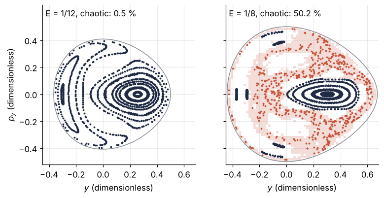
In 1964 Hénon and Heiles asked whether a star moving in a smooth galaxy has a third conserved quantity besides its energy and its angular momentum. They fixed the angular momentum as a parameter and followed the star in a plane through the galaxy's axis, so in their model the quantity sought is the second, after the energy. The answer depends on the energy, and a Poincaré section computed with solve_ivp shows it: at energy 1/8, about half of the section is chaotic.

The Hénon-Heiles model is dimensionless. The star moves in the potential \(V\) with the Hamiltonian \(H\),

\[V(x, y) = \tfrac12\left(x^2 + y^2\right) + x^2 y - \tfrac13 y^3, \qquad H = \tfrac12\left(p_x^2 + p_y^2\right) + V(x, y),\]

where \(p_x, p_y\) are the momenta. Above \(E = 1/6\), the height of the potential's three saddles, a chaotic star can escape through gaps at the saddles, so this tutorial stays at 1/12 and 1/8.

The state has four numbers, and the energy confines an orbit to a three-dimensional surface in that four-dimensional space. Record the orbit only when it crosses the line \(x = 0\) with \(p_x > 0\) and you are left with two numbers, \((y, p_y)\), because the energy gives \(p_x\) back. Every further conserved quantity removes one more dimension. If the orbit has a second one, its points on the section must lie where that quantity keeps its value, which is a closed curve. Without one, nothing holds them, and they fill an area.

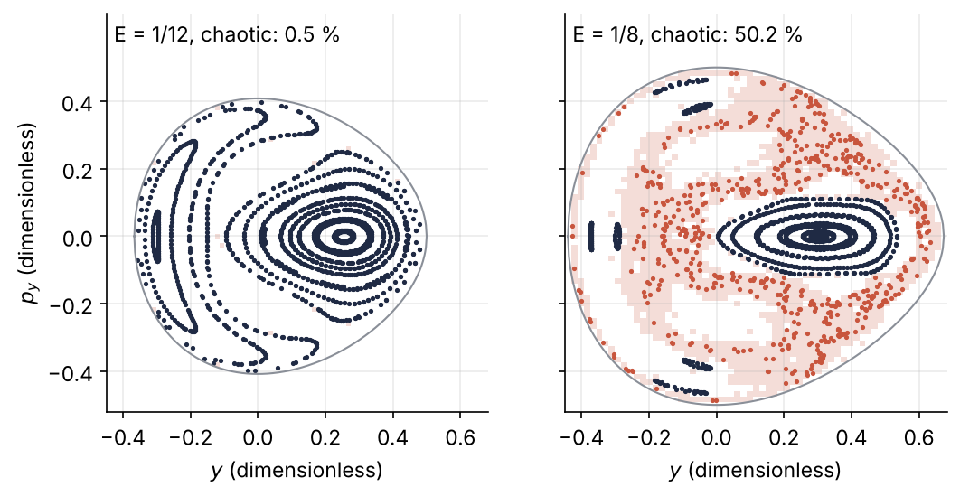
Poincaré sections of the Hénon-Heiles system at energies 1/12 and 1/8, p_y against y. At 1/12 closed curves fill the section and 0.5 % of it is chaotic; at 1/8 a shaded chaotic sea covers 50 %.

The shading is the chaotic sea, measured on a grid of about 2,700 starts per panel, each tested against a neighbor started 10⁻⁸ away. On top lie the crossings of 15 orbits, recorded with an event.

Setup

import numpy as np
import matplotlib.pyplot as plt
from scipy.integrate import solve_ivp

plt.rcParams.update({
    "figure.figsize": (7, 3.6), "figure.dpi": 110,
    "axes.spines.top": False, "axes.spines.right": False,
    "axes.grid": True, "grid.alpha": 0.25,
    "font.size": 11, "lines.linewidth": 1.8,
})
INK, ACCENT, SECOND, MUTED = "#1f2a44", "#c8553d", "#2a7f9e", "#8a8f98"

TOL = dict(method="DOP853", rtol=1e-9, atol=1e-9)   # Step 2 says why DOP853


def potential(x, y):
    return 0.5 * (x**2 + y**2) + x**2 * y - y**3 / 3


print(f"V at the saddle (0, 1) = {potential(0, 1):.6f} = 1/6, the escape energy")

V at the saddle (0, 1) = 0.166667 = 1/6, the escape energy

Step 1: Write Hamilton's equations and launch orbits on the energy surface

Hamilton's equations, \(\dot q = \partial H / \partial p\) and \(\dot p = -\partial H / \partial q\), give four first-order equations, already in the form solve_ivp wants (see solve_ivp from the ground up):

\[\dot x = p_x, \quad \dot y = p_y, \quad \dot p_x = -x - 2xy, \quad \dot p_y = -y - x^2 + y^2 .\]

Both functions below unpack the state along its first axis, so they work on one state of shape (4,) and on many states of shape (4, N), which Step 5 needs.

The launch follows a general rule. Fix the section coordinate (\(x = 0\)) and the energy, choose the two coordinates you plot (\(y, p_y\)), and solve \(H = E\) for the remaining momentum, with the sign of the crossing direction you record. Here that is \(p_x = +\sqrt{2E - p_y^2 - y^2 + 2y^3/3}\). Where the number under the root is negative, no orbit of that energy exists. The allowed region is the area inside the curve \(p_y^2 + y^2 - 2y^3/3 = 2E\), where \(p_x = 0\); this curve is the boundary of the allowed region in every figure below. The same equation has a second branch beyond \(y = 1\), which belongs to stars that have escaped.

def rhs(t, s):
    x, y, px, py = s
    return np.array([px, py, -x - 2 * x * y, -y - x**2 + y**2])


def energy(s):
    x, y, px, py = s
    return 0.5 * (px**2 + py**2) + potential(x, y)


def start(E, y, py):
    radicand = 2 * E - py**2 - y**2 + 2 * y**3 / 3
    if radicand < 0:
        raise ValueError(f"(y, p_y) = ({y}, {py}) lies outside the allowed region at E = {E}")
    return np.array([0.0, y, np.sqrt(radicand), py])


def y_range(E):
    # where the boundary crosses p_y = 0: the two roots of -y^3/3 + y^2/2 - E = 0 below y = 1
    roots = np.sort(np.roots([-1 / 3, 1 / 2, 0, -E]).real)
    return roots[0], roots[1]


for E in [1 / 12, 1 / 8]:
    lo, hi = y_range(E)
    print(f"E = {E:.4f}: allowed y on p_y = 0 from {lo:.3f} to {hi:.3f}")
s0 = start(1 / 12, 0.1, 0.0)
print("start", s0, " energy", energy(s0), " 1/12 =", 1 / 12)

E = 0.0833: allowed y on p_y = 0 from -0.366 to 0.500
E = 0.1250: allowed y on p_y = 0 from -0.440 to 0.674
start [0.         0.1        0.39665266 0.        ]  energy 0.08333333333333333  1/12 = 0.08333333333333333

At 1/12 the allowed \(y\) on the section runs from −0.366 to 0.500, at 1/8 from −0.440 to 0.674, and the start lands on its energy to the last printed digit.

The section must be crossed by every orbit you care about. Here \(\ddot x = -x(1 + 2y)\), and the allowed region stays above \(y = -1/2\), so the force always pulls \(x\) back through zero. An orbit that records no crossing means the section was badly chosen.

Step 2: Record the crossings with an event

An event function returns \(x\), and direction = 1 keeps only the crossings with \(p_x > 0\). Run one orbit at \(E = 1/12\) from \((y, p_y) = (0.1, 0)\) for 800 time units, then its first 200 again with RK45 and DOP853 to compare their cost:

def cross(t, s):
    return s[0]

cross.direction = 1     # only crossings with p_x > 0, one point per turn


def boundary(E):
    yb = np.linspace(*y_range(E), 400)
    pb = np.sqrt(np.clip(2 * E - yb**2 + 2 * yb**3 / 3, 0, None))
    return np.concatenate([yb, yb[::-1]]), np.concatenate([pb, -pb[::-1]])


sol = solve_ivp(rhs, (0, 800), start(1 / 12, 0.1, 0.0), events=cross, **TOL)
pts = sol.y_events[0]                  # one row per crossing: (x, y, p_x, p_y)
E_pts = energy(pts.T)
print(f"{len(pts)} crossings, energy spread {np.ptp(E_pts):.1e}, relative {np.ptp(E_pts) * 12:.1e}")

for method in ["RK45", "DOP853"]:
    s = solve_ivp(rhs, (0, 200), start(1 / 12, 0.1, 0.0), method=method, rtol=1e-9, atol=1e-9)
    print(f"{method:6s} nfev = {s.nfev:6d} over 200 time units")

fig, ax = plt.subplots(figsize=(4.5, 4))
ax.plot(*boundary(1 / 12), color=MUTED, lw=1)
ax.plot(pts[:, 1], pts[:, 3], "o", color=INK, ms=2)
ax.set(xlabel="$y$ (dimensionless)", ylabel="$p_y$ (dimensionless)", aspect="equal")
plt.show()

129 crossings, energy spread 3.0e-08, relative 3.7e-07
RK45   nfev =  16778 over 200 time units
DOP853 nfev =   6494 over 200 time units

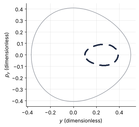
Poincaré section of one Hénon-Heiles orbit at energy 1/12, p_y against y. 129 crossings lie on a single closed curve inside the gray boundary of the allowed region.

sol.y_events[0] holds the full state at each crossing, so columns 1 and 3 are \((y, p_y)\). The energy at the 129 crossings varies by 3.0 × 10⁻⁸, a relative spread of 3.7 × 10⁻⁷ around the 1/12 we launched with. At the same tolerance RK45 needs 2.6 times as many evaluations as DOP853, an eighth-order Runge-Kutta method that SciPy recommends when you need high accuracy. That factor is paid on every orbit of this tutorial.

The 129 points lie on one closed curve. This orbit has a second conserved quantity.

Step 3: Draw the section from many orbits

One orbit draws one curve. The section is the curves of many orbits at the same energy, started on the line \(p_y = 0\) at 15 points spread over the allowed range:

def section(E, y0s, t_end=800):
    orbits = []
    for y0 in y0s:
        s = solve_ivp(rhs, (0, t_end), start(E, y0, 0.0), events=cross, **TOL)
        orbits.append(s.y_events[0][:, [1, 3]])
    return orbits


starts = {E: np.linspace(*y_range(E), 17)[1:-1] for E in [1 / 12, 1 / 8]}   # ends excluded
orbits = {E: section(E, y0s) for E, y0s in starts.items()}
for E, orb in orbits.items():
    print(f"E = {E:.4f}: {len(orb)} orbits, {sum(len(o) for o in orb)} section points")

fig, ax = plt.subplots(figsize=(5, 4))
ax.plot(*boundary(1 / 8), color=MUTED, lw=1)
for o in orbits[1 / 8]:
    ax.plot(o[:, 0], o[:, 1], "o", color=INK, ms=1.5)
ax.set(xlabel="$y$ (dimensionless)", ylabel="$p_y$ (dimensionless)", aspect="equal")
plt.show()

E = 0.0833: 15 orbits, 1913 section points
E = 0.1250: 15 orbits, 1899 section points

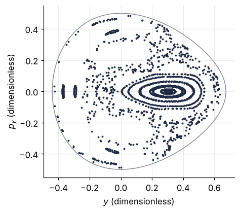
Poincaré section of 15 orbits at energy 1/8, p_y against y. Nested closed curves form islands; between them points scatter over a wide area.

At \(E = 1/8\) the section has three kinds of structure. An island is a family of nested closed curves. At its center sits a periodic orbit: a star that comes back to the same \((y, p_y)\) at every crossing, so its section is a single point. The star still moves; the section only sees it at the same place. The points scattered between the islands belong to orbits without a second conserved quantity, and that region is the chaotic sea. The eye tells the two apart; it cannot say how much area the sea covers.

Step 4: Tell chaos from regularity with a neighbor

Start a second orbit 10⁻⁸ away in \(y\), on the same energy surface (start recomputes \(p_x\)), and watch the distance between the two in the four-dimensional phase space. On a regular orbit they drift apart roughly linearly with time, because neighboring closed curves are traversed at slightly different rates. On a chaotic orbit the distance grows exponentially until it reaches the size of the allowed region.

t = np.linspace(0, 500, 501)
dist = {}
for y0 in [0.1, -0.2]:
    a = solve_ivp(rhs, (0, 500), start(1 / 8, y0, 0.0), t_eval=t, **TOL)
    b = solve_ivp(rhs, (0, 500), start(1 / 8, y0 + 1e-8, 0.0), t_eval=t, **TOL)
    dist[y0] = np.linalg.norm(a.y - b.y, axis=0)
    above = t[dist[y0] > 1e-4]
    first = f"t = {above[0]:.0f}" if above.size else "never"
    print(f"y0 = {y0:5.2f}: distance {dist[y0][-1]:.2e} at t = 500, first above 1e-4: {first}")

fig, ax = plt.subplots()
ax.semilogy(t, dist[0.1], color=INK)
ax.semilogy(t, dist[-0.2], color=ACCENT)
ax.axhline(1e-4, color=MUTED, lw=1, ls="--")
ax.text(505, dist[0.1][-1], "regular, y₀ = 0.1", color=INK, va="center")
ax.text(505, dist[-0.2][-1], "chaotic, y₀ = −0.2", color=ACCENT, va="center")
ax.text(495, 2e-4, "threshold 10⁻⁴", color=MUTED, ha="right")
ax.set(xlabel="$t$ (dimensionless)", ylabel="separation (dimensionless)", xlim=(0, 500))
plt.show()

y0 =  0.10: distance 5.62e-07 at t = 500, first above 1e-4: never
y0 = -0.20: distance 8.07e-01 at t = 500, first above 1e-4: t = 101

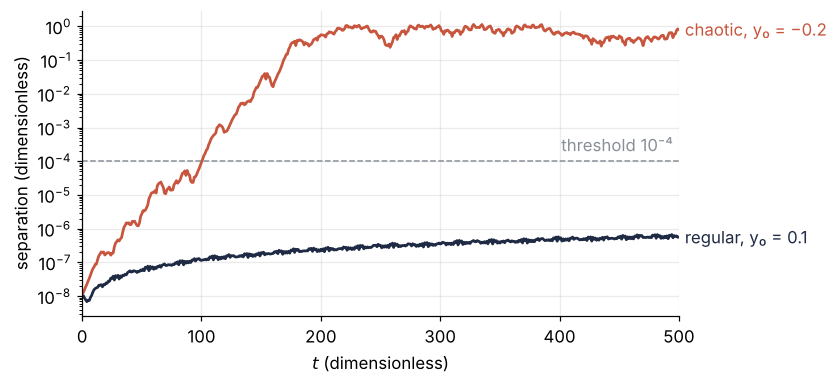
Distance between two orbits started 1e-8 apart, log scale, against time up to 500. The regular pair stays below 1e-6; the chaotic pair passes the 1e-4 threshold near t = 101 and levels off near 1, the size of the allowed region.

The regular pair is 5.6 × 10⁻⁷ apart at \(t = 500\). The chaotic pair passes 10⁻⁴ at \(t = 101\), and at \(t = 500\) the two are 0.81 apart, the size of the allowed region itself. For these two orbits a threshold of 10⁻⁴ sits more than two orders of magnitude from either, so its exact value hardly matters. The rate of the exponential growth is called the largest Lyapunov exponent. The test only asks whether it is positive.

Step 5: Integrate a whole grid of orbits in one call

Step 6 tests about 2,700 starts per energy, each with its neighbor. In separate calls that takes minutes, because most of the time goes into Python's overhead per step, not into arithmetic. One solve_ivp call with all the orbits in one state pays that overhead once per step for all of them, and NumPy does the arithmetic for all of them at once.

Put the N starts and their N neighbors as the columns of one array S of shape (4, 2N): starts in columns 0 to N − 1, neighbors in N to 2N − 1. solve_ivp wants a flat vector, so pass S.ravel(), and let rhs_many reshape it back to (4, 2N) before calling Step 1's rhs. At the end, reshape(4, 2, N) hands back starts and neighbors as two (4, N) blocks, and the distance of each pair is the norm of their difference over the first axis.

def rhs_many(t, s):
    return rhs(t, s.reshape(4, -1)).ravel()


def separation(E, ys, pys, T, dy=1e-8):
    S = np.column_stack([start(E, y, py) for y, py in zip(ys, pys)]
                        + [start(E, y + dy, py) for y, py in zip(ys, pys)])
    sol = solve_ivp(rhs_many, (0, T), S.ravel(), **TOL)
    end = sol.y[:, -1].reshape(4, 2, len(ys))
    return np.linalg.norm(end[:, 0] - end[:, 1], axis=0)


d = separation(1 / 8, [0.1, -0.2], [0.0, 0.0], 500)
print(f"N = 2, stacked state of {8 * 2} numbers")
print(f"regular {d[0]:.2e} (Step 4: {dist[0.1][-1]:.2e})   chaotic {d[1]:.2e} (Step 4: {dist[-0.2][-1]:.2e})")

N = 2, stacked state of 16 numbers
regular 5.62e-07 (Step 4: 5.62e-07)   chaotic 6.44e-01 (Step 4: 8.07e-01)

The regular distance agrees with Step 4 to the printed digits; the chaotic one does not, and cannot. All orbits in one call share one sequence of steps, chosen from an error averaged over every component, so each orbit takes slightly different steps than alone, and on a chaotic orbit that difference grows like the 10⁻⁸ offset. Both chaotic distances, 0.64 and 0.81, lie over three orders of magnitude above the threshold, which is all the test asks.

Step 6: Measure the chaotic fraction of the section

Lay a uniform 61 × 61 grid over the box around the allowed region and keep the points inside it. Each grid point stands for an equal patch of the \((y, p_y)\) plane, so the share of chaotic points is the share of the area. Integrate every start with its neighbor to \(t = 500\) and call it chaotic when the two are more than 10⁻⁴ apart:

grids = {}
for E in [1 / 12, 1 / 8]:
    lo, hi = y_range(E)
    Y, P = np.meshgrid(np.linspace(lo, hi, 61), np.linspace(-np.sqrt(2 * E), np.sqrt(2 * E), 61))
    inside = 2 * E - P**2 - Y**2 + 2 * Y**3 / 3 > 0
    chaotic = np.zeros_like(Y, dtype=bool)
    d = separation(E, Y[inside], P[inside], 500)
    chaotic[inside] = d > 1e-4
    grids[E] = (Y, P, inside, chaotic)
    print(f"E = {E:.4f}: {inside.sum()} starts, chaotic fraction {chaotic[inside].mean():.3f}"
          f" (threshold 1e-3: {(d > 1e-3).mean():.3f})")

E = 0.0833: 2767 starts, chaotic fraction 0.005 (threshold 1e-3: 0.003)
E = 0.1250: 2721 starts, chaotic fraction 0.502 (threshold 1e-3: 0.478)

At \(E = 1/12\) the chaotic fraction is 0.005, a few grid cells at the edges of islands; at \(E = 1/8\) it is 0.502. The small number is the fragile one. Chaotic starts at an island's edge separate slowly, and a threshold of 10⁻³ counts only 0.003 at \(E = 1/12\), while at \(E = 1/8\) it moves the fraction from 0.502 to 0.478. Hénon and Heiles saw curves everywhere at 1/12 and a large share of scattered points at 1/8. For their curve of area against energy they also used a neighbor, started about 10⁻⁷ away, but they summed the squared distances on the section over 25 crossings and called the sum chaotic above about 10⁻⁴: the threshold used here, on a different quantity. The final figure puts both sections side by side, each of the 15 orbits from Step 3 colored by its own test:

fig, axes = plt.subplots(1, 2, figsize=(8, 4.2), sharex=True, sharey=True)
for ax, (E, label) in zip(axes, [(1 / 12, "E = 1/12"), (1 / 8, "E = 1/8")]):
    Y, P, inside, chaotic = grids[E]
    ax.pcolormesh(Y, P, np.ma.masked_where(~chaotic, chaotic.astype(float)),
                  cmap=plt.matplotlib.colors.ListedColormap([ACCENT]), alpha=0.2,
                  shading="nearest", lw=0)
    is_chaotic = separation(E, starts[E], np.zeros_like(starts[E]), 500) > 1e-4
    for o, c in zip(orbits[E], is_chaotic):
        ax.plot(o[:, 0], o[:, 1], "o", color=ACCENT if c else INK, ms=1.5)
    ax.plot(*boundary(E), color=MUTED, lw=1)
    ax.text(0.02, 0.98, f"{label}, chaotic: {100 * chaotic[inside].mean():.1f} %",
            transform=ax.transAxes, va="top")      # in the strip above the section
    ax.set(xlabel="$y$ (dimensionless)", aspect="equal",
           ylim=(-0.52, 0.66), yticks=[-0.4, -0.2, 0, 0.2, 0.4])
axes[0].set(ylabel="$p_y$ (dimensionless)")
plt.show()

Poincaré sections of the Hénon-Heiles system at energies 1/12 and 1/8, p_y against y. At 1/12 closed curves fill the section and 0.5 % of it is chaotic; at 1/8 a shaded chaotic sea covers 50 %.

The number depends a little on how long you wait. Some chaotic orbits stick near the edge of an island: their points stay close to one closed curve for hundreds of time units before they leave for the sea, and until then the neighbor test calls them regular. Twice the time catches more of them:

Y, P, inside, chaotic = grids[1 / 8]
longer = separation(1 / 8, Y[inside], P[inside], 1000) > 1e-4
print(f"E = 0.1250: chaotic fraction {chaotic[inside].mean():.3f} at T = 500, {longer.mean():.3f} at T = 1000")

E = 0.1250: chaotic fraction 0.502 at T = 500, 0.554 at T = 1000

Five percentage points more at twice the cost. Half of the section, to a good approximation, is chaotic at \(E = 1/8\).

Pitfalls

Tolerances too loose, so a regular orbit looks chaotic. Run the orbit of Step 2 with the default tolerances for 2,000 time units:

loose = solve_ivp(rhs, (0, 2000), start(1 / 12, 0.1, 0.0), events=cross)
tight = solve_ivp(rhs, (0, 2000), start(1 / 12, 0.1, 0.0), events=cross, **TOL)
for name, s in [("defaults", loose), ("DOP853 1e-9", tight)]:
    E_ev = energy(s.y_events[0].T)
    print(f"{name:12s} {len(E_ev):4d} crossings, energy spread {100 * np.ptp(E_ev) * 12:.2g} % of E")

fig, ax = plt.subplots(figsize=(4.5, 4))
ax.plot(loose.y_events[0][:, 1], loose.y_events[0][:, 3], "o", color=ACCENT, ms=2)
ax.plot(tight.y_events[0][:, 1], tight.y_events[0][:, 3], "o", color=INK, ms=2)
ax.text(0.245, 0.02, "default tolerances", color=ACCENT, ha="center")
ax.text(0.245, -0.02, "DOP853, 10⁻⁹", color=INK, ha="center", va="top")
ax.set(xlabel="$y$ (dimensionless)", ylabel="$p_y$ (dimensionless)", aspect="equal")
plt.show()

defaults      319 crossings, energy spread 33 % of E
DOP853 1e-9   321 crossings, energy spread 9.1e-05 % of E

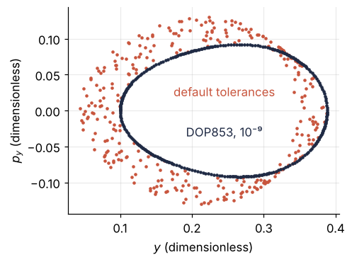
The same orbit at energy 1/12 with default and tight tolerances, p_y against y. Tight: a thin closed curve. Default: the points spread into a wide band as the energy drifts by 33 percent.

The energy drifts by a third, and the closed curve smears into a band that looks like a chaotic orbit. The section is only as good as the energy it was computed at, so print the spread of the energy at the crossings with every section you draw.

Counting crossings in both directions. Without cross.direction = 1 the event also fires when the orbit crosses \(x = 0\) with \(p_x < 0\). Those points land in the same \((y, p_y)\) plane but belong to a different section. The orbit of Step 2 then reports 257 events instead of 129, and the two curves on top of each other look like extra structure or, at higher energy, like extra chaos.

Starting outside the allowed region. A negative number under the square root of the launch gives NumPy's nan with a RuntimeWarning, and solve_ivp then stops with "All components of the initial state y0 must be finite." In the stacked call of Step 5 that message stands for one bad start among 2,700 and does not say which. Silencing it with np.abs or a clip under the root is worse: the star is launched at another energy, and nothing tells you. The check in start raises at the bad start and names it, and the inside mask of Step 6 keeps grid points outside the boundary from ever reaching it.

Variations

The standard map. A section in closed form, \((p, \theta) \mapsto (p + K\sin\theta,\ \theta + p + K\sin\theta)\), with no ODE at all. Iterate it from a grid of starts and the same islands and seas appear as \(K\) grows.
A driven pendulum. The section is stroboscopic: the state once per drive period, taken with t_eval or dense_output, as solve_ivp from the ground up sketches.
The double pendulum. Section at \(\theta_1 = 0\) with \(\dot\theta_1 > 0\), plotted in \((\theta_2, \dot\theta_2)\). The launch rule of Step 1 gives \(\dot\theta_1\) as the positive root of the energy, which is quadratic in the angular velocities. Check, as Step 1 did for \(x = 0\), that every orbit you care about crosses \(\theta_1 = 0\).
Sweep the energy. Run Step 6 at energies from 1/24 to just below 1/6 and plot the fraction against \(E\), the summary curve Hénon and Heiles drew for the area covered by closed curves.

Cheat sheet

def cross(t, s): return s[0]                       # section x = 0
cross.direction = 1                                # one direction only
sol = solve_ivp(rhs, (0, T), s0, events=cross, method="DOP853", rtol=1e-9, atol=1e-9)
pts = sol.y_events[0][:, [1, 3]]                   # (y, p_y) at each crossing
px = np.sqrt(2 * E - py**2 - 2 * potential(0, y))  # launch: remaining momentum from E
np.ptp(energy(sol.y_events[0].T))                  # energy spread: check every section
S = np.column_stack([starts, neighbors])           # (4, 2N), solved as S.ravel()
rhs_many = lambda t, s: rhs(t, s.reshape(4, -1)).ravel()
chaotic = np.linalg.norm(end[:, 0] - end[:, 1], axis=0) > 1e-4   # end = sol.y[:, -1].reshape(4, 2, N)