REBOUND from the ground up: the outer planets for a million years

The problem: will the outer planets keep their orbits for a million years?

Jupiter, Saturn, Uranus, and Neptune pull on each other all the time. Will they still be on their present orbits a million years from now, after about 84,300 turns of Jupiter? A general-purpose solver such as solve_ivp either crawls through that span or lets the energy drift. REBOUND, the standard N-body code for planetary systems, answers it with its integrator WHFast in 1.7 million steps.

WHFast is a Wisdom-Holman integrator. It splits every step into two pieces it can do exactly: a drift, in which each planet follows its Kepler ellipse around the Sun, and a kick, in which the planets' mutual pull changes their velocities. A method built this way is symplectic. For exponentially long times it conserves, to a good approximation, a nearby quantity: not the true energy, but one that differs from it by a small term set by the step. The error in the true energy therefore oscillates instead of growing (Symplectic integrators: why leapfrog's energy error is bounded and RK4's drifts shows why). It steps a twentieth of Jupiter's period at a time.

The check throughout is the total energy, kinetic plus the potential of every pair,

with \(m_i\) and \(v_i\) the mass and speed of body \(i\) and \(r_{ij}\) the distance between bodies \(i\) and \(j\). Nothing outside acts on the system, so any change in \(E\) is the integrator's doing.

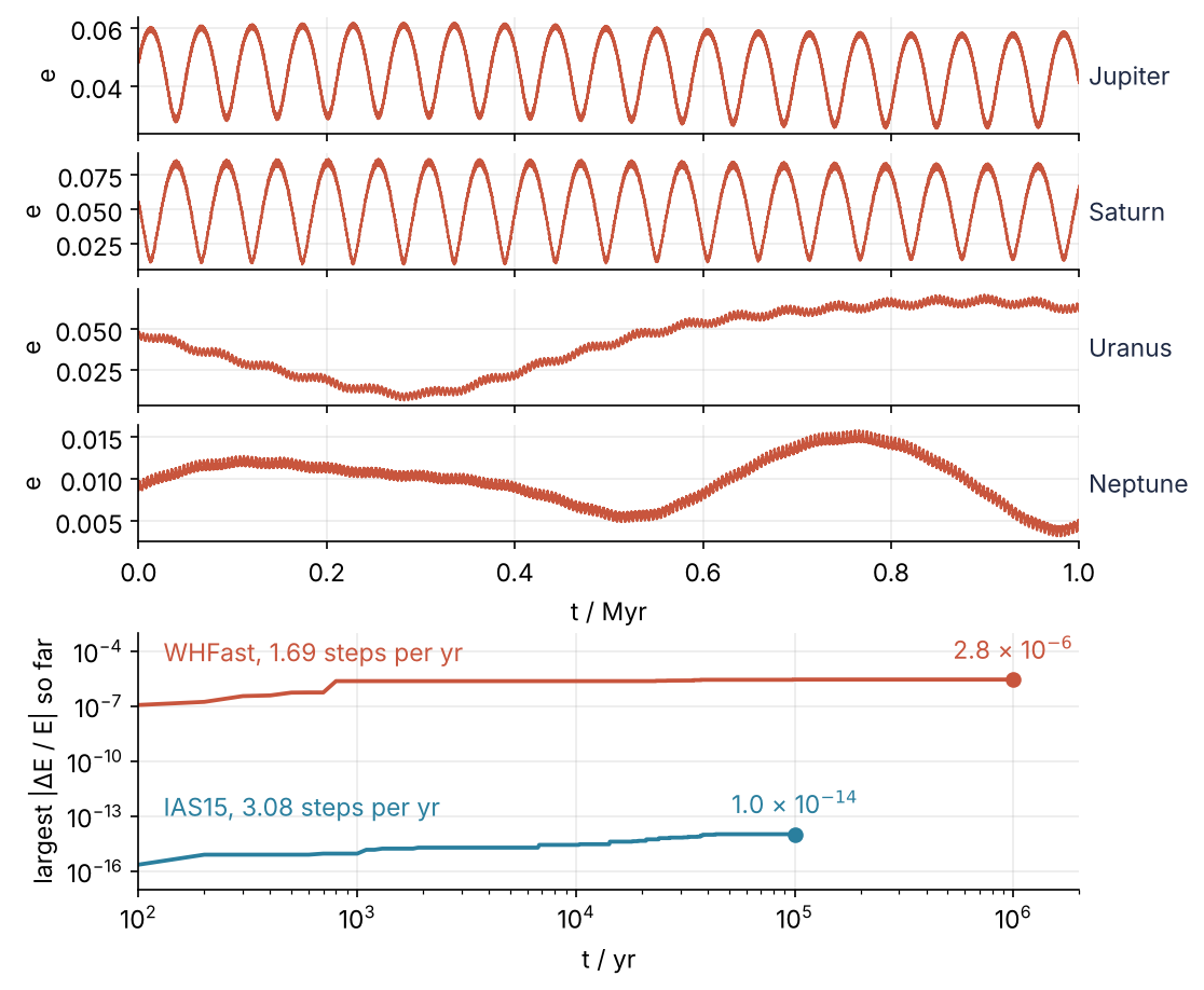
The four eccentricities swing back and forth for a million years and none of them runs away. Below, WHFast's energy error levels off at a few parts in a million, and IAS15, REBOUND's high-accuracy integrator, stays lower by a factor of 3 × 10⁸ to 3 × 10⁹ for the tenth of the span it covers. Step 5 draws it.

Setup

The numbers are the Sun and the four giant planets on 5 September 1994, from Hairer, Lubich, and Wanner, Geometric Numerical Integration (2nd ed., Springer 2006), section I.2.4: heliocentric positions in AU, velocities in AU per day, masses in solar masses. The Sun's mass includes the inner planets.

import numpy as np
import matplotlib.pyplot as plt
import rebound

NAMES = ["Jupiter", "Saturn", "Uranus", "Neptune"]
MASS = np.array([1.00000597682, 0.000954786104043, 0.000285583733151,
                 0.0000437273164546, 0.0000517759138449])          # Sun first, solar masses
POS = np.array([[0, 0, 0],
                [-3.5023653, -3.8169847, -1.5507963],
                [9.0755314, -3.0458353, -1.6483708],
                [8.3101420, -16.2901086, -7.2521278],
                [11.4707666, -25.7294829, -10.8169456]])           # AU
VEL = np.array([[0, 0, 0],
                [0.00565429, -0.00412490, -0.00190589],
                [0.00168318, 0.00483525, 0.00192462],
                [0.00354178, 0.00137102, 0.00055029],
                [0.00288930, 0.00114527, 0.00039677]])             # AU/day
G_TABLE = 2.95912208286e-4                                         # AU^3 / (Msun day^2)
DAY_PER_YR = 365.25

plt.rcParams.update({
    "figure.figsize": (7, 3.6), "figure.dpi": 110,
    "axes.spines.top": False, "axes.spines.right": False,
    "axes.grid": True, "grid.alpha": 0.25,
    "font.size": 11, "lines.linewidth": 1.8,
})
INK, ACCENT, SECOND, MUTED = "#1f2a44", "#c8553d", "#2a7f9e", "#8a8f98"

print(f"REBOUND {rebound.__version__}")

REBOUND 5.2.2

Step 1: Set up the Sun and the four giant planets

A REBOUND system is a Simulation with particles added one by one. Set the units first: REBOUND derives the gravitational constant from them and refuses to change units once particles exist. The cell then prints each planet's orbit twice. p.e is REBOUND's own eccentricity, measured around the center of mass of all bodies inside the planet's orbit; Step 2 explains why. p.orbit(primary=sim.particles[0]) returns an Orbit object with the same elements measured around the Sun alone, the heliocentric values a textbook table lists.

def outer_planets():
    sim = rebound.Simulation()
    sim.units = ("day", "AU", "Msun")
    for m, (x, y, z), (vx, vy, vz) in zip(MASS, POS, VEL):
        sim.add(m=m, x=x, y=y, z=z, vx=vx, vy=vy, vz=vz)
    return sim

sim = outer_planets()
sim.move_to_com()
print(f"G = {sim.G:.11e}   table: {G_TABLE:.11e}\n")

print("           a / AU   e (Jacobi)   e (heliocentric)   P / yr")
for name, p in zip(NAMES, sim.particles[1:]):
    e_helio = p.orbit(primary=sim.particles[0]).e
    print(f"{name:8s} {p.a:8.3f}   {p.e:10.4f}   {e_helio:16.4f}   {p.P / DAY_PER_YR:6.2f}")

G = 2.95912208286e-04   table: 2.95912208286e-04

           a / AU   e (Jacobi)   e (heliocentric)   P / yr
Jupiter     5.203       0.0484             0.0484    11.86
Saturn      9.543       0.0532             0.0526    29.46
Uranus     19.196       0.0470             0.0462    84.05
Neptune    30.073       0.0086             0.0066   164.81

The units give the table's \(G\) to every digit it prints, and Jupiter's period comes out at 11.86 years, the shortest of the four and the one that sets the time step. The eccentricities lie between 0.0086 and 0.0532. The two columns differ slightly, most for Neptune (0.0086 against 0.0066), the planet with the most mass inside its orbit besides the Sun. The same choice of center holds for p.a and p.P.

A body you know by its orbit rather than its state goes in as sim.add(m=..., a=..., e=..., primary=sim.particles[0]), which is the usual form for a system of your own; Pitfall 1 uses it. The table puts the Sun at rest at the origin, so the system as typed carries a net momentum. move_to_com shifts everything into the frame where the center of mass sits still; Pitfall 2 shows what happens without it.

Step 2: Integrate with WHFast and pick the time step

The integrator and the step are two attributes of the simulation. The helper below integrates a copy, so that sim stays at \(t = 0\), and records sim.energy() with each planet's eccentricity and semimajor axis. It calls integrate with exact_finish_time=0. A symplectic method needs the same step every time, and an exact finish would shorten the last step before each output.

The experiment runs 10⁴ years four times, halving dt from a tenth of Jupiter's period to an eightieth. If the largest energy error falls as \(\Delta t^p\), each halving divides it by \(2^p\). The ratio column is that factor, the previous run's error over this one's, so it reads off \(p\), the order of the method.

def run(sim, t_end, n_out):
    """Integrate a copy of sim to t_end (days); return n_out + 1 records and the step count."""
    sim = sim.copy()
    t = np.linspace(0, t_end, n_out + 1)
    E = np.empty(n_out + 1)
    ecc = np.empty((n_out + 1, sim.N - 1))
    a = np.empty_like(ecc)
    for k, tk in enumerate(t):
        sim.integrate(tk, exact_finish_time=0)
        E[k] = sim.energy()
        ecc[k] = [p.e for p in sim.particles[1:]]
        a[k] = [p.a for p in sim.particles[1:]]
    return t / DAY_PER_YR, np.abs(E / E[0] - 1), ecc, a, sim.steps_done

sim.integrator = "whfast"
P_J = sim.particles[1].P                      # Jupiter's period, days

print(" n    dt / day   largest |dE/E|   ratio    steps")
previous = None
for n in [10, 20, 40, 80]:
    sim.dt = P_J / n
    t, dE, ecc, a, steps = run(sim, 1e4 * DAY_PER_YR, 100)
    ratio = f"{previous / dE.max():5.2f}" if previous else ""
    print(f"{n:2d}   {sim.dt:8.1f}   {dE.max():14.2e}   {ratio:>5s}   {steps:6d}")
    previous = dE.max()

 n    dt / day   largest |dE/E|   ratio    steps
10      433.2         9.81e-06             8431
20      216.6         2.34e-06    4.20    16862
40      108.3         5.75e-07    4.06    33724
80       54.2         1.41e-07    4.06    67447

The ratios are 4.06 to 4.20, so \(p = 2\): WHFast is second order, and twice the steps buy four times the accuracy. The step for the rest of the tutorial is \(P_J/20\), 217 days, with an error of 2.3 × 10⁻⁶. The rule: start at a fraction of the shortest orbital period, then halve and check that the error falls by four.

The coordinates explain why such a large step works. WHFast measures each planet from the center of mass of the Sun and all planets inside its orbit, which are called Jacobi coordinates. In them the motion splits exactly into a Kepler orbit per planet around the mass it actually circles, and a kick that depends on positions only and is smaller than the Kepler pull by the planet-to-Sun mass ratio, about 10⁻³. They are WHFast's default (sim.integrator.coordinates reads back 'JACOBI'), and they are Step 1's first eccentricity column. Add the bodies from the inside out: the Jacobi elements of each body depend on everything added before it.

Step 3: Run a million years and record the orbital elements

A million years at one record per century is 10,001 calls to integrate, the first at \(t = 0\), and the same helper.

sim.dt = P_J / 20
t, dE, ecc, a, steps = run(sim, 1e6 * DAY_PER_YR, 10_000)

print("            e min   e mean   e max      a min / AU   a max / AU")
for k, name in enumerate(NAMES):
    print(f"{name:8s} {ecc[:, k].min():7.4f}  {ecc[:, k].mean():7.4f}  {ecc[:, k].max():6.4f}"
          f"   {a[:, k].min():10.4f}   {a[:, k].max():10.4f}")
print(f"\ncorrelation of e, Jupiter with Saturn: {np.corrcoef(ecc[:, 0], ecc[:, 1])[0, 1]:.2f}")
print(f"largest |dE/E| over 1e6 yr: {dE.max():.2e}   steps: {steps}")

            e min   e mean   e max      a min / AU   a max / AU
Jupiter   0.0254   0.0460  0.0617       5.2013       5.2049
Saturn    0.0098   0.0530  0.0871       9.5324       9.5550
Uranus    0.0057   0.0424  0.0715      19.1821      19.2070
Neptune   0.0032   0.0100  0.0158      30.0598      30.0883

correlation of e, Jupiter with Saturn: -0.96
largest |dE/E| over 1e6 yr: 2.84e-06   steps: 1686161

The largest energy error over a million years is 2.8 × 10⁻⁶, barely above the 2.3 × 10⁻⁶ of the 10⁴-year run, as a symplectic method promises. The semimajor axes stay within a quarter of a percent of their starting values. The eccentricities wander much more: Saturn's between 0.0098 and 0.0871, Uranus's between 0.0057 and 0.0715. That is secular evolution, the slow change driven by the other planets' pull averaged over their orbits, on time scales of tens of thousands of years and longer. Through that averaged pull the planets trade eccentricity, so one rises while another falls: Jupiter's and Saturn's have a correlation of −0.96.

The sampling interval is not arbitrary. Five Jupiter periods, 59.3 years, almost equal two Saturn periods, 58.9 years, so their mutual pull repeats with the beat period \(1/(5/P_S - 2/P_J)\), near 900 years, the great inequality. A record every 1,000 years would catch that oscillation at almost the same phase each time and draw a slow wave that is not there, which is called aliasing. Every 100 years resolves it.