Symplectic integrators: why leapfrog's energy error is bounded and RK4's drifts (Python)

The question

A frictionless pendulum released from 1 rad swings forever with the same amplitude, because its energy

\[H(q, p) = \tfrac12 p^2 + 1 - \cos q\]

never changes. Here \(q\) is the angle and \(p\) the angular velocity, in units where \(g/L = 1\), so time counts in units of \(\sqrt{L/g}\). It starts with \(H_0 = 0.4597\) and swings with a period of 6.70. Integrate it with five one-step methods at \(h = 0.1\) and watch what each does to \(H\).

Explicit Euler follows the slopes at the start of the step, implicit Euler those at the end, at the cost of an equation per step. RK4 is the classical fourth-order Runge-Kutta method. The other two split the step into a kick, which changes \(p\) with the force at the current \(q\), and a drift, which moves \(q\) with the current \(p\). Symplectic Euler is one kick, then one drift,

\[p_{n+1} = p_n - h \sin q_n, \qquad q_{n+1} = q_n + h\, p_{n+1},\]

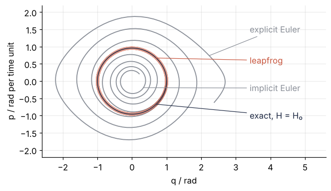
and leapfrog is a half kick, a drift, and another half kick: the scheme of velocity Verlet under another name. Here are 250 steps of three of them in the phase plane, computed by the tutorial's own code, with the curve \(H = H_0\) that the exact pendulum never leaves.

Show code

import numpy as np
import matplotlib.pyplot as plt

plt.rcParams.update({
    "figure.figsize": (7, 3.6), "figure.dpi": 110,
    "axes.spines.top": False, "axes.spines.right": False,
    "axes.grid": True, "grid.alpha": 0.25,
    "font.size": 11, "lines.linewidth": 1.8,
})
INK, ACCENT, SECOND, MUTED = "#1f2a44", "#c8553d", "#2a7f9e", "#8a8f98"

# Units with g/L = 1: time in units of sqrt(L/g), p is the angular velocity in units of sqrt(g/L).
def H(q, p):
    return 0.5 * p**2 + 1 - np.cos(q)

def pendulum(q):                  # the force and its derivative, the latter for implicit Euler's Newton loop
    return -np.sin(q), -np.cos(q)

def oscillator(q):
    return -q, -np.ones_like(q)

def explicit_euler(q, p, h=0.1, force=pendulum):
    f, _ = force(q)
    return q + h * p, p + h * f

def implicit_euler(q, p, h=0.1, force=pendulum):
    Q = q + h * p                 # the explicit guess, then Newton on Q = q + h (p + h f(Q))
    for _ in range(6):
        f, df = force(Q)
        Q = Q - (Q - q - h * p - h**2 * f) / (1 - h**2 * df)
    return Q, p + h * force(Q)[0]

def rk4(q, p, h=0.1, force=pendulum):
    def rhs(q, p):
        return p, force(q)[0]
    k1 = rhs(q, p)
    k2 = rhs(q + h / 2 * k1[0], p + h / 2 * k1[1])
    k3 = rhs(q + h / 2 * k2[0], p + h / 2 * k2[1])
    k4 = rhs(q + h * k3[0], p + h * k3[1])
    return (q + h / 6 * (k1[0] + 2 * k2[0] + 2 * k3[0] + k4[0]),
            p + h / 6 * (k1[1] + 2 * k2[1] + 2 * k3[1] + k4[1]))

def symplectic_euler(q, p, h=0.1, force=pendulum):
    p = p + h * force(q)[0]       # kick with the old position
    return q + h * p, p           # drift with the new momentum

def leapfrog(q, p, h=0.1, force=pendulum):
    p = p + h / 2 * force(q)[0]   # half kick
    q = q + h * p                 # drift
    return q, p + h / 2 * force(q)[0]

def run(step, q, p, n, **kw):
    """n steps from (q, p); arrays of shape (n + 1, ...) with the start in row 0."""
    qs, ps = [q], [p]
    for _ in range(n):
        q, p = step(q, p, **kw)
        qs.append(q)
        ps.append(p)
    return np.array(qs), np.array(ps)

methods = {"explicit Euler": explicit_euler, "implicit Euler": implicit_euler, "RK4": rk4,
           "symplectic Euler": symplectic_euler, "leapfrog": leapfrog}
q0, p0, N = 1.0, 0.0, 100_000
H0 = H(q0, p0)
a, b = 1.0, np.cos(q0 / 2)                  # exact period T = 2π / AGM(1, cos(q0/2)), the arithmetic-geometric mean
for _ in range(6):
    a, b = (a + b) / 2, np.sqrt(a * b)
T = 2 * np.pi / a
print(f"H₀ = {H0:.4f}, period T = {T:.2f}: 250 steps of h = 0.1 are {25 / T:.1f} periods, {N:,} steps are {N * 0.1 / T:,.0f}")
long_runs = {name: run(step, q0, p0, N) for name, step in methods.items()}
q, p = long_runs["implicit Euler"]                  # the residual of q_{n+1} = q_n + h p_{n+1} at every step
print(f"implicit Euler, largest Newton residual in {N:,} steps: {np.abs(q[1:] - q[:-1] - 0.1 * p[1:]).max():.1e}")
rel_err = {name: (H(q, p) - H0) / H0 for name, (q, p) in long_runs.items()}

fig, ax = plt.subplots()
qg, pg = np.meshgrid(np.linspace(-3.2, 3.2, 400), np.linspace(-2.2, 2.2, 400))
for name in ["explicit Euler", "implicit Euler"]:
    ax.plot(long_runs[name][0][:251], long_runs[name][1][:251], color=MUTED, lw=1.2)
q, p = long_runs["leapfrog"][0][:251], long_runs["leapfrog"][1][:251]
ax.plot(q, p, color=ACCENT, lw=4, alpha=0.6)            # wide, so that the exact curve shows inside it
ax.contour(qg, pg, H(qg, pg), levels=[H0], colors=INK, linewidths=1)
p_on_curve = np.sqrt(2 * (H0 - 1 + np.cos(0.7)))         # a point of H = H₀ at q = 0.7, for the leader lines
for text, xy, xytext, color in [
        ("explicit Euler", [a[225] for a in long_runs["explicit Euler"]], (3.4, 1.5), MUTED),
        ("leapfrog", (0.7, p_on_curve), (3.4, 0.6), ACCENT),
        ("implicit Euler", [a[200] for a in long_runs["implicit Euler"]], (3.4, -0.2), MUTED),
        ("exact, H = H₀", (0.7, -p_on_curve), (3.4, -1.0), INK)]:
    ax.annotate(text, xy, xytext=xytext, color=color, va="center",
                arrowprops=dict(arrowstyle="-", lw=0.8, color=color, shrinkA=2, shrinkB=0))
ax.set(xlabel="q / rad", ylabel="p / rad per time unit", aspect="equal", xlim=(-2.6, 5.6), ylim=(-2.2, 2.2))
plt.show()

top = np.argmax(H(*long_runs["explicit Euler"]) > 2)
print(f"\n{'':17s}  ΔH/H₀ at step 250   largest |ΔH/H₀| in 1,000 steps   in {N:,} steps")
for name, r in rel_err.items():
    if name == "explicit Euler":
        print(f"{name:17s}  {r[250]:+17.2e}   past the top (H > 2) from step {top}")
    else:
        print(f"{name:17s}  {r[250]:+17.2e}   {np.abs(r[:1001]).max():29.2e}   {np.abs(r).max():15.2e}")

H₀ = 0.4597, period T = 6.70: 250 steps of h = 0.1 are 3.7 periods, 100,000 steps are 1,493
implicit Euler, largest Newton residual in 100,000 steps: 6.2e-17

Phase plane of the pendulum, p against q in rad, 250 steps of h = 0.1 from q = 1, p = 0. Explicit Euler spirals outward, implicit Euler spirals inward, leapfrog stays on the exact closed curve.

                   ΔH/H₀ at step 250   largest |ΔH/H₀| in 1,000 steps   in 100,000 steps
explicit Euler             +3.16e+00   past the top (H > 2) from step 266
implicit Euler             -9.04e-01                        1.00e+00          1.00e+00
RK4                        -2.36e-06                        1.02e-05          9.97e-04
symplectic Euler           -7.26e-03                        4.92e-02          4.92e-02
leapfrog                   -2.27e-03                        2.31e-03          2.31e-03

Explicit Euler spirals outward, its energy up by 316 % at step 250, and at step 266 the pendulum goes over the top. Implicit Euler spirals inward, 90 % of its energy gone, as if the pivot had friction. Leapfrog sits on the exact curve. The table runs all five for \(10^5\) steps, 1,493 periods.

The obvious explanation is order. A method of order \(k\) has an error proportional to \(h^k\) over a fixed time: halve the step and RK4's error shrinks sixteenfold, Euler's twofold. The Euler methods are first order, leapfrog second, RK4 fourth, and at step 250 RK4's energy is off by \(2.4 \times 10^{-6}\), a thousand times less than leapfrog's.

The last two columns disagree. Symplectic Euler, first order, reaches its worst error, \(4.9 \times 10^{-2}\), within 1,000 steps and never exceeds it in the next 99,000. Leapfrog does the same at \(2.3 \times 10^{-3}\). RK4's error is a hundred times larger after \(10^5\) steps than after \(10^3\), and still growing. Why does a first-order method's energy error stop growing while a fourth-order method's keeps going?

The idea: follow a patch of pendulums, not one

One trajectory cannot tell a careful method from a lucky one. A patch of neighboring starts can. Take every pendulum whose starting point lies within 0.3 of \((1, 0)\) in the phase plane, a disk of them, and carry the whole disk with the method. The exact motion of a system like the pendulum, whose equations come from an energy function, moves the disk around and shears it out of shape, but never changes its area. That is Liouville's theorem; the Formalization shows why it holds in one line.

To measure the area I put 500 points on the boundary circle at equal angles, carry them, and take the area of the polygon through them. Here is the disk at steps 0, 60, and 120, from light to dark, under explicit Euler, symplectic Euler, and implicit Euler, with the exact disk at step 120 as an outline:

Show code

def area(q, p):
    """Shoelace area of the polygon through the points (q[i], p[i]), in order."""
    return 0.5 * abs(q @ np.roll(p, -1) - p @ np.roll(q, -1))

phi = np.linspace(0, 2 * np.pi, 500, endpoint=False)
q_disk, p_disk = 1 + 0.3 * np.cos(phi), 0.3 * np.sin(phi)
A0 = area(q_disk, p_disk)
exact_q, exact_p = run(leapfrog, q_disk, p_disk, 12_000, h=0.001)   # the exact flow, to plotting accuracy

fig, axes = plt.subplots(1, 3, figsize=(8, 2.7), sharex=True, sharey=True, layout="constrained")
for ax, name in zip(axes, ["explicit Euler", "symplectic Euler", "implicit Euler"]):
    color = ACCENT if name == "symplectic Euler" else MUTED
    q, p = run(methods[name], q_disk, p_disk, 120)
    ax.contour(qg, pg, H(qg, pg), levels=8, colors=MUTED, linewidths=0.5, alpha=0.5)
    for n, alpha in [(0, 0.2), (60, 0.35), (120, 0.6)]:        # light to dark: steps 0, 60, 120
        ax.fill(q[n], p[n], color=color, alpha=alpha, lw=0)
    ax.plot(np.append(exact_q[-1], exact_q[-1][0]), np.append(exact_p[-1], exact_p[-1][0]), color=INK, lw=1.2)
    ax.text(0.03, 0.04, f"{name}\narea × {area(q[120], p[120]) / A0:.4f}", transform=ax.transAxes,
            va="bottom", color=INK)
    ax.set(aspect="equal", xlabel="q / rad", xlim=(-2.2, 1.5), ylim=(-0.55, 1.75))
axes[0].set_ylabel("p / rad per time unit")
plt.show()

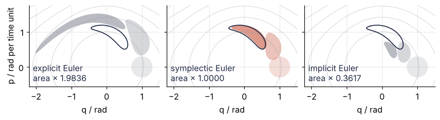
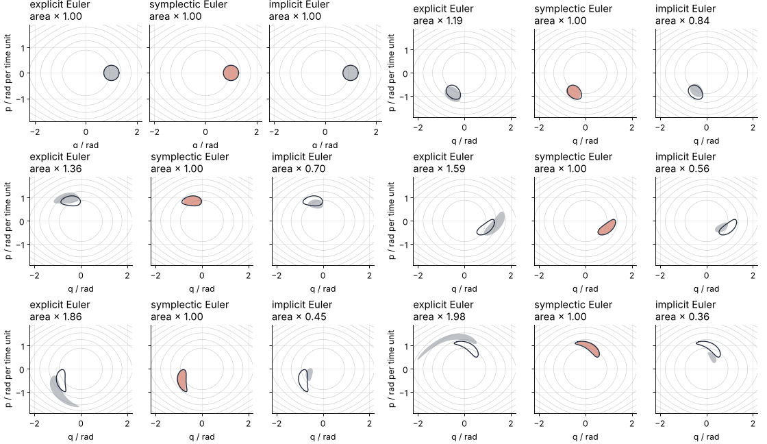
Three phase-plane panels, p against q in rad: a disk of pendulums after 0, 60, and 120 steps. Under explicit Euler the disk smears outward to 1.98 times its area, under symplectic Euler it matches the exact outline at 1.0000, under implicit Euler it shrinks to 0.36.

After 120 steps, a little under two periods, explicit Euler's disk covers 1.98 times its starting area and implicit Euler's 0.36. Symplectic Euler's reads 1.0000 and lies on the exact outline. The animation runs the same three methods one step per frame:

Three disks of pendulums in the phase plane, carried one step per frame by explicit Euler, symplectic Euler, and implicit Euler, each panel with the exact disk as a moving outline. Watch the area printed above each panel: it grows on the left, stays 1.00 in the middle, shrinks on the right.

Show code

"""A disk of pendulums carried by three one-step methods: the area grows, stays, shrinks.

Renders ../../assets/disk-flow.gif. Run it from any directory:

    python scene.py
"""
from pathlib import Path

import numpy as np
import matplotlib.pyplot as plt
from matplotlib.animation import FuncAnimation, PillowWriter
from PIL import Image

OUT = Path(__file__).resolve().parents[2] / "assets" / "disk-flow.gif"
INK, ACCENT, MUTED = "#1f2a44", "#c8553d", "#8a8f98"
plt.rcParams.update({"axes.spines.top": False, "axes.spines.right": False,
                     "axes.grid": True, "grid.alpha": 0.25, "font.size": 11})
h, STEPS, HOLD = 0.1, 120, 8                        # HOLD still frames at the start and at the end

# ---- the pendulum, H = p²/2 + 1 - cos q, and three of the tutorial's step functions
def explicit_euler(q, p):
    return q + h * p, p - h * np.sin(q)

def symplectic_euler(q, p):
    p = p - h * np.sin(q)
    return q + h * p, p

def implicit_euler(q, p):
    Q = q + h * p                                   # Newton on Q = q + h (p - h sin Q)
    for _ in range(6):
        Q = Q - (Q - q - h * p + h**2 * np.sin(Q)) / (1 + h**2 * np.cos(Q))
    return Q, p - h * np.sin(Q)

def exact(q, p):                                    # one step of h as 100 leapfrog steps: the exact flow, to plotting accuracy
    for _ in range(100):
        p = p - h / 200 * np.sin(q)
        q = q + h / 100 * p
        p = p - h / 200 * np.sin(q)
    return q, p

def area(q, p):                                     # shoelace formula on the boundary points
    return 0.5 * abs(q @ np.roll(p, -1) - p @ np.roll(q, -1))

# ---- the disk of radius 0.3 around (1, 0), as 500 boundary points, carried STEPS steps
phi = np.linspace(0, 2 * np.pi, 500, endpoint=False)
disk = (1 + 0.3 * np.cos(phi), 0.3 * np.sin(phi))
A0 = area(*disk)
panels = [("explicit Euler", explicit_euler, MUTED), ("symplectic Euler", symplectic_euler, ACCENT),
          ("implicit Euler", implicit_euler, MUTED)]
paths = []                                          # paths[0] is the exact flow, then one per panel
for step in [exact] + [step for _, step, _ in panels]:
    q, p = disk
    states = [(q, p)]
    for _ in range(STEPS):
        q, p = step(q, p)
        states.append((q, p))
    paths.append(states)

# ---- figure, drawn once
fig, axes = plt.subplots(1, 3, figsize=(7, 2.7), dpi=80, sharex=True, sharey=True, layout="constrained")
qg, pg = np.meshgrid(np.linspace(-2.2, 2.2, 300), np.linspace(-1.9, 1.9, 300))
patches, outlines, titles = [], [], []
for ax, (name, _, color) in zip(axes, panels):
    ax.contour(qg, pg, 0.5 * pg**2 + 1 - np.cos(qg), levels=8, colors=MUTED, linewidths=0.5, alpha=0.5)
    (patch,) = ax.fill(*disk, color=color, alpha=0.55, lw=0)
    (outline,) = ax.plot([], [], color=INK, lw=1.2)  # the exact disk, drawn over the method's
    patches.append(patch)
    outlines.append(outline)
    titles.append(ax.set_title("", loc="left"))
    ax.set(aspect="equal", xlabel="q / rad", xlim=(-2.2, 2.2), ylim=(-1.9, 1.9))
axes[0].set_ylabel("p / rad per time unit")

# ---- one frame: the first and the last HOLD frames repeat the start and the end
def update(frame):
    n = min(max(frame - HOLD, 0), STEPS)
    q_exact, p_exact = paths[0][n]
    for patch, outline, title, states, (name, _, _) in zip(patches, outlines, titles, paths[1:], panels):
        q, p = states[n]
        patch.set_xy(np.column_stack([q, p]))
        outline.set_data(np.append(q_exact, q_exact[0]), np.append(p_exact, p_exact[0]))
        title.set_text(f"{name}\narea × {area(q, p) / A0:.2f}")

# ---- render, and read back what was written
OUT.parent.mkdir(exist_ok=True)
FuncAnimation(fig, update, frames=2 * HOLD + STEPS + 1).save(OUT, writer=PillowWriter(fps=12))
plt.close(fig)
with Image.open(OUT) as im:
    seconds = 0.0
    for i in range(im.n_frames):                    # Pillow merges identical frames, so delays differ
        im.seek(i)
        seconds += im.info["duration"] / 1000
    print(f"{OUT.name}: {im.width} x {im.height} px, {im.n_frames} frames, "
          f"{seconds:.1f} s, {OUT.stat().st_size / 1024:,.0f} kB")

The symplectic disk is drawn out into a crescent, and that is not the method's error: the exact outline has the same shape. Pendulums near the inner edge of the disk have less energy, swing with a shorter period, and run ahead of those on the outer edge. Symplectic Euler shears the disk as the true motion does and leaves its area alone. An area that grows means the pendulums have moved, on the whole, to curves of higher energy, which is the outward spiral of the question seen for a crowd instead of a single pendulum.

Why a kick and a drift keep the area

Symplectic Euler is two shears in a row. The kick changes \(p\) by \(-h \sin q\), an amount set by \(q\) alone, so every point moves vertically and all points with the same \(q\) move by the same amount. A thin vertical strip of states slides up or down as a whole and keeps its width and height, and a patch made of such strips keeps its area, whatever the force. The drift does the same sideways: it changes \(q\) by \(h p\), an amount set by \(p\) alone. Each shear keeps area, so any sequence of them does.

Explicit Euler updates both coordinates from the old state, \(q_{n+1} = q_n + h p_n\) and \(p_{n+1} = p_n - h \sin q_n\). Its drift uses the old \(p\), not the kicked one, so the step is not a kick followed by a drift. For the harmonic oscillator, \(H = \tfrac12(p^2 + q^2)\), whose exact motion rotates the phase plane at constant speed, one explicit Euler step multiplies \((q, p)\) by the matrix \(\begin{pmatrix} 1 & h \\ -h & 1 \end{pmatrix}\). Its two columns are perpendicular and both of length \(\sqrt{1 + h^2}\), so the step is a rotation followed by a stretch by \(\sqrt{1 + h^2}\) in every direction.

Implicit Euler takes both slopes at the new state, \(q_{n+1} = q_n + h p_{n+1}\) and \(p_{n+1} = p_n - h \sin q_{n+1}\), so the unknowns stand on both sides. Substituting the second into the first leaves one equation for \(Q = q_{n+1}\),

\[Q = q_n + h\,(p_n - h \sin Q),\]

which no rearranging solves for \(Q\). Every step solves it numerically, with six Newton iterations from the explicit guess, which leave a residual of at most \(6.2 \times 10^{-17}\) over the \(10^5\) steps, the size of rounding. For the oscillator the rule shrinks every direction by \(1/\sqrt{1 + h^2}\): the mirror image of explicit Euler, and the inward spiral of the question. The same damping is what makes implicit Euler useful on stiff problems.

Here is a unit square of oscillator states under a kick and then a drift, and beside it the same square under one explicit Euler step. The step is \(h = 0.5\), five times the tutorial's, so that the effect is large enough to see:

Show code

h_big = 0.5                                       # large on purpose, so the effect is visible
square_q, square_p = np.array([0.0, 1.0, 1.0, 0.0]), np.array([0.0, 0.0, 1.0, 1.0])
kick_q, kick_p = square_q, square_p - h_big * square_q
drift_q, drift_p = kick_q + h_big * kick_p, kick_p
euler_q, euler_p = explicit_euler(square_q, square_p, h=h_big, force=oscillator)

fig, (ax1, ax2) = plt.subplots(1, 2, figsize=(7, 3.4), sharex=True, sharey=True, layout="constrained")
for ax in (ax1, ax2):
    ax.fill(square_q, square_p, facecolor="none", edgecolor=INK, lw=1.4)
    ax.text(0, 1.06, f"square: {area(square_q, square_p):.2f}", color=INK, va="bottom")
    ax.set(aspect="equal", xlabel="q (dimensionless)", xlim=(-0.2, 2.1), ylim=(-0.75, 1.45))
ax1.fill(kick_q, kick_p, color=MUTED, alpha=0.35, lw=0)
ax1.fill(drift_q, drift_p, color=ACCENT, alpha=0.4, lw=0)
ax1.text(1.05, -0.6, f"kick: {area(kick_q, kick_p):.2f}", color=MUTED)
ax1.text(1.3, 0.5, f"then drift:\n{area(drift_q, drift_p):.2f}", color=ACCENT, va="center")
ax2.fill(euler_q, euler_p, color=MUTED, alpha=0.35, lw=0)
ax2.text(1.55, 0.5, f"explicit\nEuler:\n{area(euler_q, euler_p):.2f}", color=MUTED, va="center")
ax2.text(2.05, 1.4, f"h = {h_big}", color=INK, ha="right", va="top")
ax1.set_ylabel("p (dimensionless)")
plt.show()

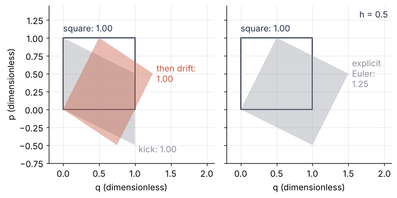
Two panels at h = 0.5, p against q. Left: a unit square, slanted by a kick and then by a drift, area 1.00 after each. Right: the same square after one explicit Euler step, turned and enlarged to area 1.25.

The kick slants the square into a parallelogram of the same base and height, the drift slants that one sideways, and both read 1.00. One explicit Euler step of the same size turns the square and enlarges it to 1.25, which is \(1 + h^2\). Leapfrog is three shears, half kick, drift, half kick, so it keeps area too. RK4 blends four slopes into one update that is no sequence of shears, and nothing forces its area factor to be exactly 1.

Formalization

A Hamiltonian system is one whose equations of motion come from a single function \(H(q, p)\):

\[\dot q = \frac{\partial H}{\partial p}, \qquad \dot p = -\frac{\partial H}{\partial q}.\]

A one-step method is a map \(\Phi_h\) that takes \((q_n, p_n)\) to \((q_{n+1}, p_{n+1})\). Its Jacobian \(D\Phi_h\), the 2 × 2 matrix of derivatives of the new state with respect to the old, multiplies the area of a small patch around a point by \(\det D\Phi_h\). The exact flow keeps area because its velocity field \((\partial H/\partial p,\, -\partial H/\partial q)\) has zero divergence: the two mixed second derivatives of \(H\) cancel. That is Liouville's theorem.

Definition. In two dimensions a map is symplectic when \(\det D\Phi_h = 1\) at every point. With \(d\) positions and \(d\) momenta the condition is

\[D\Phi_h^{T}\, J\, D\Phi_h = J, \qquad J = \begin{pmatrix} 0 & I \\ -I & 0 \end{pmatrix},\]

where \(J\) is the matrix of Hamilton's equations themselves, \(\dot x = J \nabla H\) for \(x = (q, p)\). It says that the sum of the areas projected onto the pairs \((q_i, p_i)\) is kept. Worked out from the step's formulas at a general state, this condition is the test that settles it for your problem. Every kick and every drift passes it, whatever \(H\).

A check on the oscillator. On the oscillator all five methods are linear maps, and the Jacobian is the step's matrix, the same at every state:

Show code

h = 0.1
identity = np.eye(2)
closed_form = {"explicit Euler": "1 + h²", "implicit Euler": "1/(1 + h²)"}
for name, step in methods.items():
    D = np.array(step(identity[0], identity[1], force=oscillator))   # columns: images of (1, 0) and (0, 1)
    det = np.linalg.det(D)
    print(f"{name:17s} det = {det:.10f}   det - 1 = {det - 1:+.3e}   {closed_form.get(name, '')}")

explicit Euler    det = 1.0100000000   det - 1 = +1.000e-02   1 + h²
implicit Euler    det = 0.9900990099   det - 1 = -9.901e-03   1/(1 + h²)
RK4               det = 0.9999999861   det - 1 = -1.387e-08   
symplectic Euler  det = 1.0000000000   det - 1 = +0.000e+00   
leapfrog          det = 1.0000000000   det - 1 = -1.110e-16

Symplectic Euler and leapfrog read 1 to rounding. Explicit Euler's 1.01 and implicit Euler's 0.990099 are \(1 + h^2\) and \(1/(1 + h^2)\), the squares of the stretches above. For RK4, one step on a linear system is the Taylor series of the exact step, a rotation, cut after the fourth power of \(h\); the cut leaves the determinant short of 1 by \(h^6/72\) to leading order, \(1.387 \times 10^{-8}\) here. Each of these three is a rotation times a scaling, so the energy changes per step by the same factor as the area. The check can rule a method out but not in: the trapezoidal rule reads 1 on the oscillator and is not symplectic on the pendulum.

The bridge to energy. Every Hamiltonian flow keeps area, so a map that changes area is not the flow of any energy function, and its \(H\) is free to drift. Backward error analysis goes the other way, approximately: a symplectic method of order \(k\), at a fixed step \(h\), follows the exact flow of a nearby Hamiltonian

\[\tilde H = H + h^k H_k + h^{k+1} H_{k+1} + \dots\]

The agreement holds up to an error exponentially small in \(1/h\), over times exponentially long in \(1/h\). So the numerical points stay on a level curve of \(\tilde H\), and \(H\) can swing by the gap \(H - \tilde H\), of order \(h^k\), but cannot drift. For leapfrog on the oscillator the kept quantity is \(\tfrac12 p^2 + \tfrac12 (1 - h^2/4)\, q^2\), exactly. For leapfrog on the pendulum,

\[\tilde H = H + \frac{h^2}{24}\left(2 p^2 \cos q - \sin^2 q\right) + O(h^4).\]

Show code

q, p = run(leapfrog, 1.0, 0.0, 1000, force=oscillator)
H_tilde_osc = 0.5 * p**2 + 0.5 * (1 - h**2 / 4) * q**2
print(f"oscillator, leapfrog, 1,000 steps: spread of H~ = {np.ptp(H_tilde_osc):.1e}")

q, p = long_runs["leapfrog"]
H_tilde = H(q, p) + h**2 / 24 * (2 * p**2 * np.cos(q) - np.sin(q)**2)
swing_H = np.abs(H(q, p) - H0).max() / H0
swing_H_tilde = np.abs(H_tilde - H_tilde[0]).max() / H0
print(f"pendulum, leapfrog, {N:,} steps: largest |ΔH/H₀| = {swing_H:.2e}, "
      f"largest |ΔH~/H₀| = {swing_H_tilde:.2e}, ratio {swing_H / swing_H_tilde:.0f}")

oscillator, leapfrog, 1,000 steps: spread of H~ = 2.1e-15
pendulum, leapfrog, 100,000 steps: largest |ΔH/H₀| = 2.31e-03, largest |ΔH~/H₀| = 3.94e-06, ratio 586

Symplectic is not energy-conserving. Over \(10^5\) steps leapfrog's \(H\) swings by up to \(2.31 \times 10^{-3}\) of \(H_0\) and its \(\tilde H\) by \(3.94 \times 10^{-6}\), 586 times less. The oscillator's quadratic varies by \(2.1 \times 10^{-15}\) over 1,000 steps, which is rounding.

Bounded energy, growing phase. On the oscillator leapfrog's step matrix has determinant 1 and trace \(2 - h^2\), so it turns by the angle whose cosine is half the trace, \(\arccos(1 - h^2/2) = 1.000417\, h\) per step instead of \(h\):

Show code

q, p = run(leapfrog, 1.0, 0.0, N, force=oscillator)
t = h * np.arange(N + 1)
ahead = np.unwrap(np.arctan2(-p, q))[-1] - t[-1]   # the exact solution turns by exactly t
energy = np.abs(0.5 * (q**2 + p**2) - 0.5).max() / 0.5
print(f"angle per step: {np.arccos(1 - h**2 / 2) / h:.6f} h")
print(f"after {N:,} steps: {ahead:.2f} rad ahead of the exact solution, energy within {100 * energy:.2f} %")

angle per step: 1.000417 h
after 100,000 steps: 4.17 rad ahead of the exact solution, energy within 0.25 %

After \(10^5\) steps it is 4.17 rad ahead of the exact solution, two thirds of a turn, with the energy still within 0.25 %. The phase error grows linearly, without limit. A bounded energy says nothing about where on its orbit the pendulum is.

The step must be fixed in advance. With a step \(h(q)\) chosen from the state, the drift moves each point by \(h(q)\, p\), an amount set by \(q\) as well as \(p\), and it is no longer a shear. Compare it with a step that varies as much on a schedule fixed before the run:

Show code

def energy_error(step_size):
    """Leapfrog on the pendulum from (1, 0), the step chosen by step_size(n, q) before each step."""
    q, p, err = 1.0, 0.0, []
    for n in range(N):
        q, p = leapfrog(q, p, h=step_size(n, q))
        err.append(abs(H(q, p) - H0) / H0)
    return np.max(err[:1000]), np.max(err)

print("largest |ΔH/H₀|               first 1,000 steps   all 100,000 steps")
for label, step_size in [("step from the state, 0.1 (1 + 0.5 cos q)", lambda n, q: 0.1 * (1 + 0.5 * np.cos(q))),
                         ("step fixed in advance, 0.1 (1 + 0.5 sin 0.37 n)", lambda n, q: 0.1 * (1 + 0.5 * np.sin(0.37 * n)))]:
    first, overall = energy_error(step_size)
    print(f"{label}\n{'':30s} {first:13.2e} {overall:19.2e}")

largest |ΔH/H₀|               first 1,000 steps   all 100,000 steps
step from the state, 0.1 (1 + 0.5 cos q)
                                    6.36e-03            1.11e+00
step fixed in advance, 0.1 (1 + 0.5 sin 0.37 n)
                                    1.16e-02            1.16e-02

The step chosen from the state starts out better, \(6.4 \times 10^{-3}\) after 1,000 steps, and ends at 1.11, an error larger than the starting energy. The scheduled step composes symplectic maps and stays at \(1.16 \times 10^{-2}\) from the first 1,000 steps to the last. solve_ivp chooses every step from an error estimate, that is, from the state. Never put an adaptive step under a symplectic method and expect the bound to survive.

See it in code

The cell carries the disk with all five methods and measures its area with the shoelace formula on the 500 boundary points, \(A = \tfrac12 \left| \sum_i (q_i\, p_{i+1} - p_i\, q_{i+1}) \right|\). For the oscillator the answer must be \(\det^n\). Last, it finds when RK4's drift leaves leapfrog's band: at three step sizes it divides leapfrog's largest energy swing by RK4's drift per step, the slope of a straight line through its error:

Show code

print("pendulum disk, area after n steps / area at start")
for name, step in methods.items():
    q, p = run(step, q_disk, p_disk, 1000)
    print(f"  {name:17s}" + "".join(f"   n = {n}: {area(q[n], p[n]) / A0:9.4f}" for n in [100, 300, 1000]))

# The same disk for the oscillator, where every map is a matrix and the area must be det^n
osc_ratio, dets = {}, {}
for name in ["explicit Euler", "implicit Euler", "RK4", "leapfrog"]:
    q, p = run(methods[name], q_disk, p_disk, 1000, force=oscillator)
    osc_ratio[name] = np.array([area(qi, pi) for qi, pi in zip(q, p)]) / A0
    dets[name] = np.linalg.det(np.array(methods[name](identity[0], identity[1], force=oscillator)))
print("\noscillator disk after 1,000 steps: area ratio, and det^1000")
for name in osc_ratio:
    print(f"  {name:17s} {osc_ratio[name][-1]:12.6g}   {dets[name]**1000:12.6g}")

# Where RK4's drift leaves leapfrog's band, measured at three step sizes
print("\n     h   leapfrog bound   RK4 drift per step   crossing / steps   / periods")
rows = []
for h_s, n_s in [(0.05, 100_000), (0.1, 100_000), (0.2, 50_000)]:
    if h_s == 0.1:
        r_lf, r_rk = rel_err["leapfrog"], rel_err["RK4"]
    else:
        r_lf = (H(*run(leapfrog, 1.0, 0.0, n_s, h=h_s)) - H0) / H0
        r_rk = (H(*run(rk4, 1.0, 0.0, n_s, h=h_s)) - H0) / H0
    bound = np.abs(r_lf).max()
    drift = np.polyfit(np.arange(n_s + 1), r_rk, 1)[0]
    print(f"  {h_s:4.2f}   {bound:14.2e}   {drift:18.2e}   {bound / abs(drift):16.2e}   {bound / abs(drift) * h_s / T:9,.0f}")
    rows.append((bound, drift))
(b1, d1), (b2, d2), (b3, d3) = rows
print(f"per doubling of h: bound × {b2 / b1:.2f}, × {b3 / b2:.2f};  drift per step × {d2 / d1:.1f}, × {d3 / d2:.1f}")

fig, (ax1, ax2) = plt.subplots(1, 2, figsize=(8, 3.6), layout="constrained")
n = np.arange(1001)
ax1.plot(n, osc_ratio["explicit Euler"], color=MUTED)
ax1.plot(n, osc_ratio["implicit Euler"], color=MUTED)
ax1.plot(n, osc_ratio["RK4"], color=SECOND, lw=3)
ax1.plot(n, osc_ratio["leapfrog"], color=ACCENT, lw=1.4)
ax1.text(560, 2e3, "explicit Euler", color=MUTED, ha="right", va="bottom")
ax1.text(560, 5e-4, "implicit Euler", color=MUTED, ha="right", va="top")
ax1.text(1000, 2.5, "leapfrog: 1", color=ACCENT, ha="right", va="bottom")
ax1.text(1000, 0.4, f"RK4: {osc_ratio['RK4'][-1]:.6f}", color=SECOND, ha="right", va="top")
ax1.set(yscale="log", xlabel="step n", ylabel="area / initial area", xlim=(0, 1000))

r_lf, r_rk = 1e3 * rel_err["leapfrog"], 1e3 * rel_err["RK4"]   # in units of 10⁻³
blocks = r_lf[1:].reshape(-1, 100)                  # min and max per 100 steps keep the band light
steps = np.arange(1, N + 1, 100)
ax2.fill_between(steps, blocks.min(axis=1), blocks.max(axis=1), color=ACCENT, alpha=0.30, lw=0)
ax2.axhline(-np.abs(r_lf).max(), color=MUTED, ls="--", lw=1)
ax2.plot(np.arange(N + 1), r_rk, color=SECOND)
ax2.text(N, r_rk[-1] - 0.06, f"RK4: {r_rk[-1]:.3f}".replace("-", "−"), color=SECOND, ha="right", va="top")
ax2.text(0.03 * N, -np.abs(r_lf).max() + 0.06, f"leapfrog: down to −{np.abs(r_lf).max():.2f}",
         color=ACCENT, va="bottom")
ax2.xaxis.set_major_formatter(lambda x, _: f"{x:,.0f}")
ax2.set(xlabel="step n", ylabel="ΔH / H₀ / 10⁻³", xlim=(0, N), xticks=np.linspace(0, N, 5),
        ylim=(-2.6, 0.15))
plt.show()

pendulum disk, area after n steps / area at start
  explicit Euler      n = 100:    1.8978   n = 300:   34.0143   n = 1000:  637.0344
  implicit Euler      n = 100:    0.4351   n = 300:    0.0650   n = 1000:    0.0001
  RK4                 n = 100:    1.0000   n = 300:    1.0000   n = 1000:    0.9996
  symplectic Euler    n = 100:    1.0000   n = 300:    1.0000   n = 1000:    0.9993
  leapfrog            n = 100:    1.0000   n = 300:    1.0000   n = 1000:    0.9996

oscillator disk after 1,000 steps: area ratio, and det^1000
  explicit Euler         20959.2        20959.2
  implicit Euler     4.77118e-05    4.77118e-05
  RK4                   0.999986       0.999986
  leapfrog                     1              1

     h   leapfrog bound   RK4 drift per step   crossing / steps   / periods
  0.05         5.77e-04            -1.56e-10           3.70e+06      27,598
  0.10         2.31e-03            -9.97e-09           2.32e+05       3,456
  0.20         9.24e-03            -6.27e-07           1.47e+04         439
per doubling of h: bound × 4.00, × 4.00;  drift per step × 63.9, × 62.9

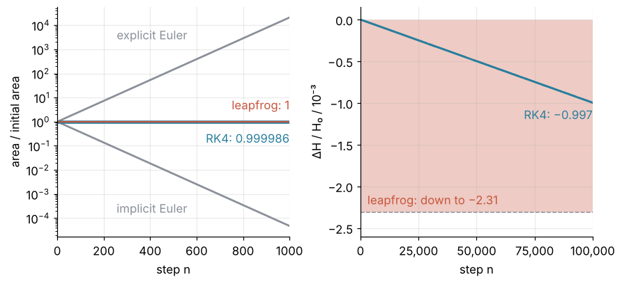
Left: area of a disk of oscillator states over 1,000 steps, relative to its start, log scale. Explicit Euler grows to 2e4, implicit Euler falls to 5e-5, RK4 and leapfrog stay at 1. Right: pendulum energy error over 1e5 steps, a flat band for leapfrog, a straight line for RK4.

For the oscillator the area after 1,000 steps equals \(\det^{1000}\) to every printed digit, 20,959.2 for explicit Euler and \(4.77 \times 10^{-5}\) for implicit Euler, because a linear map takes a polygon to a polygon. On the pendulum the symplectic methods read 1.0000 at 300 steps, and so does RK4, whose loss, \(1.4 \times 10^{-8}\) per step on the oscillator, no four-digit area can show. The shortfall at 1,000 steps, down to 0.9993, is the polygon failing to follow a boundary stretched into a filament, not the methods.

On the right, RK4's error is a line and leapfrog's a band that does not widen. The table says when the line leaves the band: at \(h = 0.1\) after \(2.32 \times 10^5\) steps, 3,456 periods. Its last line is the measured law: per doubling of \(h\) the bound grows fourfold, as \(h^2\), and the drift per step about 64-fold, as \(h^6\). The oscillator explains the sixth power: there RK4 loses \(h^6/72\) of its energy per step. The pendulum has its own constant. So the crossing moves as \(h^{-4}\), and halving the step keeps RK4 ahead sixteen times longer. One RK4 step costs four force evaluations to leapfrog's one, so at equal cost leapfrog runs at a quarter of the step, with a band sixteen times narrower. For your own simulation, run both methods for a few thousand steps and divide leapfrog's largest swing by RK4's drift per step. The result is a number of steps; plan more than that, and the symplectic method wins.

Where it shows up

The pendulum is the smallest case of a problem that runs through physics and chemistry: a Hamiltonian system followed for far more periods than any error estimate was built for.

Molecular dynamics. GROMACS, LAMMPS, and most other molecular dynamics codes move the atoms with velocity Verlet or leapfrog at a fixed step of 1 to 2 fs, for runs of \(10^8\) steps and more. Bond lengths are held fixed by a constraint algorithm, LINCS by default in GROMACS, or SHAKE and RATTLE, which keep the scheme symplectic when their iterations converge.
Planetary orbits. The Wisdom-Holman mapping of 1991 splits the solar system's Hamiltonian into Kepler motion around the Sun, solved exactly as a drift, and the planets' pulls on each other, applied as kicks. REBOUND's WHFast implements it, and integrations of this kind over millions of years are how the long-term stability of planetary systems is studied.
Particle accelerators. A beam in a storage ring is tracked for millions of turns with one symplectic map per element of the ring, each magnet a kick and each straight section a drift. A non-symplectic map would invent damping or growth of the beam that the machine does not have.
Hamiltonian Monte Carlo. Stan and PyMC propose the next sample by running leapfrog on a fictitious Hamiltonian whose potential energy is the negative log density. Volume preservation and reversibility make the Metropolis acceptance a ratio of densities, and the bounded energy error keeps the acceptance rate high over long trajectories.
Plasma physics. The Boris pusher, the standard step for a charged particle in a magnetic field, keeps phase-space volume but is in general not symplectic, as Qin and coworkers showed in 2013. Volume alone does not bound its energy error: Hairer and Lubich proved in 2018 that the error stays bounded in a uniform magnetic field and can drift in a general one.

What carries over to all of them is one rule: a method that meets the symplectic condition at a fixed step keeps its energy error bounded, whatever its order. With one degree of freedom that condition is keeping phase-space area; with more it asks more than keeping volume, which is why the Boris pusher can drift.

The question

The idea: follow a patch of pendulums, not one

Why a kick and a drift keep the area

Formalization

See it in code

Where it shows up

Further reading