The Saha equation with brentq: the temperature at which hydrogen recombined (Python)

The problem

Hydrogen's ionization energy, $\chi$ = 13.6 eV, equals $kT$ at 158,000 K, yet the early universe's hydrogen stayed ionized until it had cooled to a few thousand kelvin. Photons outnumber baryons 1.6 billion to one, so even the rare ones far in the Wien tail outnumber the atoms, and a free electron has far more room than a bound one. You want the temperature at which half the hydrogen is ionized, found with brentq as in the root-finding tutorial, and its redshift from $T = T_0(1 + z)$. The example uses $T_0 = 2.7255$ K today and $\eta = 6.1 \times 10^{-10}$ baryons per photon; swap in your own density. The Saha equation, ionization and recombination in balance, says where it tips:

\[ \frac{n_e n_p}{n_{H^0}} = n_Q\, e^{-\chi/kT}, \qquad n_Q = \left(\frac{m_e kT}{2\pi\hbar^2}\right)^{3/2}, \]

\[ n_e = n_p = x\, n_H,\quad n_{H^0} = (1 - x)\, n_H \quad\Longrightarrow\quad \frac{x^2}{1 - x} = S(T) = \frac{n_Q}{n_H}\, e^{-\chi/kT}, \]

\[ n_H = \eta\, n_\gamma, \qquad n_\gamma = \frac{2\zeta(3)}{\pi^2}\left(\frac{kT}{\hbar c}\right)^3 . \]

The code

import numpy as np
import matplotlib.pyplot as plt
from scipy import constants as sc
from scipy.optimize import brentq
from scipy.special import zeta

# ---- constants, SI throughout
k, hbar, c, m_e, m_p = sc.k, sc.hbar, sc.c, sc.m_e, sc.m_p
T0 = 2.7255                                       # CMB temperature today, K

# ---- your gas: hydrogen; another gas only with one ionization stage, see The knobs
chi = sc.Rydberg * sc.h * c * m_p / (m_p + m_e)   # 13.598 eV: Rydberg energy, reduced-mass corrected
g_factor = 1.0                                    # 2 g+ / g0 from the statistical weights; 1 for hydrogen
eta = 6.1e-10                                     # baryons per photon, from the CMB

def n_H(T):                                       # hydrogen nuclei per m^3: put your own density here
    return eta * n_gamma(T)

# ---- Saha equation
def n_gamma(T):                                   # photons per m^3, the Planck spectrum integrated
    return 2 * zeta(3) / np.pi**2 * (k * T / (hbar * c))**3

def n_Q(T):                                       # quantum concentration of electrons, per m^3
    return (m_e * k * T / (2 * np.pi * hbar**2))**1.5

def saha_S(T):                                    # right-hand side of x^2 / (1 - x) = S
    return g_factor * n_Q(T) / n_H(T) * np.exp(-chi / (k * T))

def ionized_fraction(T):                          # root of x^2 + S x - S = 0, with nothing subtracted
    S = saha_S(T)
    return 2 * S / (S + np.sqrt(S**2 + 4 * S))

# ---- half ionization
T_half, res = brentq(lambda T: ionized_fraction(T) - 0.5, 2000, 10000, full_output=True)
assert res.converged
z_half = T_half / T0 - 1

# ---- report and plot
print(f"photons per baryon     {1 / eta:.2e}")
print(f"n_Q/n_gamma at T_half  {n_Q(T_half) / n_gamma(T_half):.2e}")
print(f"T_half  = {T_half:7.1f} K")
print(f"kT_half = {k * T_half / sc.eV:7.3f} eV, chi/kT = {chi / (k * T_half):.1f}")
print(f"z_half  = {z_half:7.1f}")
print(f"brentq: {res.function_calls} function calls")

z = np.linspace(800, 1800, 801)
x = ionized_fraction(T0 * (1 + z))
fig, ax = plt.subplots(figsize=(7, 4), dpi=110)
ax.plot(z, x, color="#1f2a44", lw=1.8)
ax.axvline(1090, color="#8a8f98", lw=1, ls="--")
ax.text(1080, 0.55, "last scattering\n(Planck satellite)", color="#8a8f98", ha="left", va="center")
ax.plot(z_half, 0.5, "o", color="#c8553d", ms=6, zorder=3)
ax.annotate(f"x = 1/2 at z = {z_half:,.0f}\nT = {T_half:,.0f} K", (z_half, 0.5), (z_half - 40, 0.75),
            color="#c8553d", arrowprops=dict(arrowstyle="-", color="#c8553d", lw=0.8))
ax.set(xlim=(1800, 800), ylim=(-0.02, 1.02),      # z backward: the universe cools from left to right
       xlabel="redshift z", ylabel="ionized fraction x")
ax.spines[["top", "right"]].set_visible(False)
plt.show()

photons per baryon     1.64e+09
n_Q/n_gamma at T_half  5.16e+08
T_half  =  3759.6 K
kT_half =   0.324 eV, chi/kT = 42.0
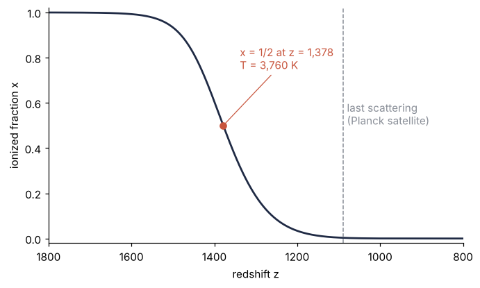
z_half  =  1378.4
brentq: 12 function calls

$Ionized fraction x of hydrogen against redshift z, with z falling from 1,800 on the left to 800 on the right as the universe cools. x drops from near 1 to near 0 and crosses 1/2 at z = 1,378 (3,760 K), well before the dashed last-scattering line at z = 1,090.$

The knobs

Half ionization means $S = 1/2$, so $e^{\chi/kT}$ must equal $2n_Q/n_H = 2\,(1/\eta)\,(n_Q/n_\gamma)$: the number of states open to a freed electron for every atom, against the Boltzmann advantage of the bound one. Both factors are in the output. The photon count, $1/\eta = 1.64 \times 10^9$, has a logarithm of 21, and it is what the Wien tail $e^{-\chi/kT}$ is weighed against. The electron's room, $n_Q/n_\gamma = 5.16 \times 10^8$, has a logarithm of 20: at the same temperature a thermal electron carries $\sqrt{m_e c^2/kT} \approx$ 1,260 times the momentum of a thermal photon (511 keV over 0.324 eV), so it has about $1{,}260^3 \approx 2 \times 10^9$ times the room in momentum space, and $n_Q/n_\gamma = 0.26\,(m_e c^2/kT)^{3/2}$. The two are halves of one reason, and neither alone gives the printed $\chi/kT = 42$: their product with the 2 is $1.7 \times 10^{18}$, whose logarithm is 42. Because $\eta$ sits inside that logarithm, ten times more baryons only moves $T_{1/2}$ to 3,987 K ($z$ = 1,462), ten times fewer to 3,557 K ($z$ = 1,304), and helium as a neutral spectator, $n_H = (1 - Y)\,\eta\, n_\gamma$ with $Y = 0.245$, lowers it to 3,734 K ($z$ = 1,369). For hydrogen at a fixed density, return a constant from n_H and widen the bracket to [3,000, 30,000] K: at $10^{22}$ m⁻³, the order of magnitude of a stellar photosphere, half ionization comes at 11,830 K. Another gas needs its own chi and g_factor $= 2g_+/g_0$ (4 from neutral helium to He⁺, with $\chi$ = 24.6 eV), and the quadratic holds only while one ionization stage supplies all the free electrons; a mixture is a coupled problem this code does not solve.

Saha assumes equilibrium, which holds only while recombination is fast compared with the expansion. In the early universe it is not: Lyman-alpha photons re-excite their neighbors, and the full calculation (Peebles' three-level atom, RECFAST and its successors) recombines later than Saha and freezes out at a residual ionization of order $10^{-4}$, where Saha drives $x$ to zero. Last scattering, the moment the universe became transparent, is near $z$ = 1,090, where Saha already gives $x$ = 0.0033. So 3,760 K is a first estimate and an upper bound on the redshift of recombination, not last scattering.

Pitfalls

The textbook quadratic formula. Written as $x = (-S + \sqrt{S^2 + 4S})/2$, the root subtracts two nearly equal numbers when $S$ is large. Here $S$ reaches $2.7 \times 10^{10}$ at 10,000 K, and above 7,500 K the formula returns $x$ = 1.0 exactly at most temperatures and up to $2 \times 10^{-6}$ off, either way, at the rest. The neutral fraction $1 - x$, $3.7 \times 10^{-11}$ at 10,000 K, is lost in that noise. In thinner gas, with larger $S$, it gets worse: up to 6 % off for $S$ below $10^{15}$, then $x$ = 0, 1, 2, or 4 for a fully ionized gas from $S = 10^{16}$, and $x$ = 0 every time above $S = 10^{17}$. Use $2S/(S + \sqrt{S^2 + 4S})$, the same root with nothing subtracted, and take the neutral fraction from the equation itself, $x^2/S$, never as $1 - x$. The floating-point tutorial shows the same cancellation.

nan below a few hundred kelvin. Extend the temperature grid toward today's 2.7 K, and $x$ comes back nan with RuntimeWarning: invalid value encountered in divide. Below 212 K, $\chi/kT$ exceeds 745 and $e^{-\chi/kT}$ underflows to 0, so $S$ is exactly 0 and the stable formula computes 0/0. Flipping the sign to divide by $e^{+\chi/kT}$ does not help: it overflows to inf below 222 K, giving the same $S = 0$ and nan. Keep the grid where the physics happens, above 2,000 K here, where $x$ is still $10^{-8}$. If you need the wide grid, write $x = 2/(1 + \sqrt{1 + 4/S})$, the same root, which returns 0 for $S = 0$, and silence its divide-by-zero warning with np.errstate(divide="ignore").

Electronvolts against joules. Set chi = 13.6 in eV while k is in J/K, and $\chi/kT$ comes out near $10^{20}$ at any temperature. Then $x$ is nan everywhere, for the reason above, and brentq stops with ValueError: The function value at x=2000.0 is NaN; solver cannot continue. Keep SI throughout, convert an energy once with scipy.constants.eV, and print $kT$ in eV at the end: 0.324 eV for a few thousand kelvin is the check.